

Updates
June 2025: Unjournal Review
The Unjournal have published a very positive independent review of this report. Learn more about the review and our response to it.
Summary
Mental health disorders like depression and anxiety are common and severely impact subjective wellbeing. Mental healthcare is poorly funded in low income countries, making it a largely neglected problem. Fortunately, a low cost solution exists. Psychotherapy effectively treats depression and anxiety, and it can be delivered relatively cheaply by lay (i.e., non-specialist) counsellors.
This report presents an in-depth cost-effectiveness evaluation of two charities delivering such lay-delivered talk psychotherapy in Africa: Friendship Bench and StrongMinds. This forms part of our broader work to assess the cost-effectiveness of interventions and charities based on their impact on subjective wellbeing, measured in terms of wellbeing-adjusted life years (WELLBYs). One WELLBY is equivalent to a 1-point increase on a 0-10 wellbeing scale for one person over one year.
We focus on subjective wellbeing because it is what ultimately matters in determining if someone’s life is going well. By using wellbeing as a common outcome, it allows to make apples-to-apples comparisons between very different interventions.
We report the cost-effectiveness of these interventions in terms of WELLBYs per $1,000 donated to the organisation (‘WBp1k’), and, conversely, the cost for each organisation to produce one WELLBY. We estimate that:
- Friendship Bench has a cost-effectiveness of 49 WBp1k, or $21 per WELLBY.
- StrongMinds has a cost-effectiveness of 40 WBp1k, or $25 per WELLBY.
We have estimated the cost-effectiveness of GiveDirectly to be only 7.55 WBp1k (i.e., $132 per WELLBY) using a meta-analysis (McGuire et al., 2022a). GiveDirectly is an NGO which provides cash transfers to very poor households. We take cash transfers as a useful benchmark because they are a straightforward, plausibly cost-effective intervention with a solid evidence base.
Our results show that both psychotherapy interventions are roughly 5-6x more cost-effective than cash transfers at improving people’s subjective wellbeing. (For more detailed and updated charity comparisons, see our charity evaluations page.)
This is the fourth iteration of our analysis, reflecting several years of research and refinement to ensure rigorous and reliable evaluations. These updates are not routine, but driven by new data and methodological improvements that strengthen our confidence in the findings, ensuring that donors and decision-makers receive the most accurate, actionable insights available. We explain how this version builds on the previous ones at the end of the summary.
Our conclusion that these two organisations are the most cost-effective and well-evidenced charities we have evaluated to date has not changed since the last version.
In the rest of this summary, we briefly present our methodology, detailed results for the charities, and a history of the different versions of this analysis. For those interested in diving deeper into the technical rigour behind our conclusion, the rest of the report offers comprehensive explanations of the methods and findings. For methodologically-minded readers, we also include an extensive 165 page appendix to give the fine details of our analysis. We encourage readers whose questions are not addressed in the summary to consult the full report and/or appendix, as we have likely addressed similar concerns there.
Methods
For each charity, we have three sources of evidence we can use to estimate the effect of the programme:
- Our own expanded and improved meta-analysis of 84 randomised controlled trials (RCTs) of psychotherapy in low and middle income countries (LMICs).
- RCTs of programmes related to the charities (4 for Friendship Bench and 1 for StrongMinds).
- Monitoring and Evaluation (‘M&E’) pre-post data from the charities themselves.
Each of these sources presents a qualitatively distinct, but potentially informative, piece of evidence to draw upon.
This is how we analysed each source of evidence. We:
- Estimated the initial effect and duration, in order to calculate the total effect for the recipient over time.
- Adjusted the total effect to account for concerns about:
- internal validity (e.g., publication bias)
- external validity (e.g., the relevance of the evidence to how the charity delivers the programme in practice).
- Estimated household spillovers to estimate the overall benefit for the recipient and their household.
We then calculate a final effect estimate for each charity by combining the three estimates from different evidence sources, using informed subjective weights. Finally, we calculate the cost-effectiveness by pairing the estimated effect for each charity with the estimated cost to deliver the intervention.
We also consider the following elements in determining our confidence in our cost-effectiveness estimates:
- Depth of analysis.
- Quality of evidence: We assess quality of evidence according to an adapted version of the ‘GRADE’ criteria, a widely-used and rigorous tool for assessing evidence quality across healthcare and research fields. The GRADE criteria for evidence quality are very stringent, so we expect very few interventions that we evaluate for wellbeing in LMICs (which tend to be less well-studied) will score more than ‘moderate’ on the quality of their evidence.
- Robustness: We made the analytical choices that we consider to be the most appropriate. Nevertheless, we explore how robust our results are to other analytical choices which we think are less appropriate but may be plausible to others.
- Site visits: We conducted site visits to both Friendship Bench and StrongMinds, which reassured us that they were operating professional and effective programmes. While we do not think site visits inform us much about cost-effectiveness, they are an important part of due diligence.
Friendship Bench
Friendship Bench is a charity operating in Zimbabwe that treats people with common mental health disorders (e.g., depression and anxiety) using a type of psychotherapy called problem-solving therapy. Friendship Bench’s standard programme consists of 1-6 sessions of individual counselling, which are delivered by trained community health workers.
We estimate that Friendship Bench has an overall effect of 0.80 WELLBY, and costs $16.50 to treat one client. This leads to a cost-effectiveness of 49 WBp1k, or a cost per WELLBY of $21. This is 6.4 times more cost-effective than cash transfers.
Our analysis was ‘in-depth’, which means we believe we have reviewed most or all of the relevant available evidence on the topic, and we have completed nearly all (e.g., 90%+) of the analyses we think are useful.
This is one of the most well-evidenced interventions we have evaluated to date. That being said, based on our stringent GRADE-adapted criteria, we rate the quality of evidence for Friendship Bench to be ‘low to moderate’. This means there is more uncertainty about the effects than if high(er) quality evidence were available. This should be seen as reflecting how little excellent data there is for charity evaluations in LMICs, not on Friendship Bench in particular. As mentioned previously, we expect few interventions that we evaluate in LMICs will have more than ‘moderate’ quality evidence.
Despite this uncertainty, we find Friendship Bench is still more cost-effective than the benchmark of GiveDirectly – even if we had applied more conservative analytic choices throughout our analysis rather than using the choices we think are most plausible (we present these robustness checks in Section 9.3).
Our biggest uncertainty is that on average, recipients attended only 1.12 sessions out of the 6 possible sessions, which is very low attendance (or dosage). Although we apply an adjustment to account for this, it is lower than we would expect. That being said, the programme is still plausibly cost-effective, despite the low attendance (see Section 5.2.3 for more detail) because:
- The first psychotherapy session is actively therapeutic, and guides participants through a complete problem-solving cycle (i.e., it is not just an orientation).
- The first session involves psychoeducation (i.e., teaching participants about mental health), which can be particularly useful in LMICs where awareness of mental health issues tends to be limited.
- The results are still more cost-effective than cash transfers, even if we apply the most stringent adjustment to account for the low attendance.
Our confidence would increase with further high quality studies, evaluations of why clients attend few sessions, or improvements in participant attendance. We have also discussed this with Friendship Bench, who have told us that they have planned future external monitoring and evaluating of their programme.
StrongMinds
StrongMinds provides group interpersonal psychotherapy (IPT) for people struggling with depression. The core programme uses lay community health workers to deliver group IPT in 90-minute weekly sessions over six weeks, primarily in Uganda and Zambia.
We estimate that StrongMinds has an overall effect of 1.80 WELLBYs, and costs $44.56 to treat one client. This leads to a cost-effectiveness of 40 WBp1k, or a cost per WELLBY of $25. This is 5.3 times more cost-effective than cash transfers.
StrongMinds’ programme is more expensive but also more effective than Friendship Bench. Hence, the overall cost-effectiveness of the charities is very similar.
Our analysis was ‘in-depth’, which means we believe we have reviewed most or all of the relevant available evidence on the topic, and we have completed nearly all (e.g., 90%+) of the analyses we think are useful.
This is also one of the most well-evidenced interventions we have evaluated to date. That being said, we rate the quality of evidence for StrongMinds to be ‘low to moderate’ based on our stringent GRADE-adapted criteria. This means there is more uncertainty about the effects than if high(er) quality evidence were available. Again, we think this reflects on how little good data there is, not on StrongMinds specifically. We expect few interventions that we evaluate in LMICs will have more than moderate quality evidence.
Despite this uncertainty, StrongMinds would remain more cost-effective than GiveDirectly even if we had applied more conservative analytic choices rather than using the choices we think are most plausible and correct – except for one analytical choice, which we do not consider plausible (explained below). We present these robustness checks in Section 9.3.
There is only one randomised control trial involving StrongMinds (i.e., a working paper by Baird et al., 2024) and this finds only very small effects compared to the other evidence sources. If one puts 100% of the weight on Baird et al., instead of the other sources, this reduces the cost-effectiveness to 6.95 WBp1k (this is just below, but close to, cash transfers).
However, despite the trial taking place in Uganda (where StrongMinds operates) and using a version of StrongMinds’ model, there are several ways in which the Baird et al. study is different from StrongMinds’ actual programme in the field today, which means we cannot generalise from it as much as one might expect.
Stated succinctly (see Section 3.2.2), the RCT was a pilot from 2019 of the first time StrongMinds had implemented their programme via a partner organisation (BRAC), the first time they had worked with adolescents, and the first time they had used youth facilitators (StrongMinds primarily does therapy for adults led by adults). The facilitators were inexperienced and given insufficient supervision. Attendance was low, with 44% of participants failing to attend any sessions. Furthermore, the long-term data collection overlapped with COVID. These issues are noted by Baird et al. (2024) and/or StrongMinds themselves (StrongMinds, 2024).
Hence, despite this study being, at first glance, an RCT of StrongMinds’ programme, we do not think it is very informative about StrongMinds own operations today. We give an appreciable, but limited, weight to this source of evidence: 20% of the total, with the remaining 80% coming from the meta-analysis and the monitoring and evaluation data (see Section 7).
Our confidence in our estimate of StrongMinds’ cost-effectiveness would increase with further high quality, relevant RCTs. We have discussed this with StrongMinds and a more relevant RCT is in the works.
Comparison to previous versions of the report
This report is the fourth iteration of our analysis. Our updates over time have been driven by new data and methodological improvements which have strengthened our confidence in the findings.
Readers may be interested to know that the emergence of wellbeing – or WELLBY – cost-effectiveness analysis is very recent, with all attempts we know of (either for charities or government policies) having happened in the last 5 years. We are the first organisation to have conducted these analyses in low-income countries, and also the first to have performed systematic reviews and meta-analysis of any intervention in terms of wellbeing. We hope others - and ourselves(!) - can learn from our processes and methods and, in the future, produce analyses in fewer versions.
Here, extremely briefly, is an account of various versions (see Appendix A for more detail):
- Version 1 was our first meta-analysis of psychotherapy in LMICs and wellbeing cost-effectiveness analysis of StrongMinds (McGuire & Plant, 2021a; McGuire & Plant, 2021b).
- In Version 2 (McGuire et al., 2022b), we added ‘household spillovers’ (i.e., the impact that receiving cash or therapy had on partners and children).
- In Version 3 (McGuire et al., 2023), we made a large update by overhauling our analysis with a systematic review of psychotherapy in LMICs with 74 studies after exclusion of outliers (the V1-V2 meta-analysis was not a fully systematic review). We also added a cost-effectiveness analysis of Friendship Bench, and paid extra attention to internal and external validity adjustments (publication bias, dosage, etc.).
Our cost-effectiveness estimates changed between Version 3 and Version 4 in the following ways:
- StrongMinds increased from 30 to 40 WBp1k.
- Friendship Bench decreased from 58 to 49 WBp1k. And we have upgraded the depth of our analysis of Friendship Bench from ‘shallow’ to ‘in-depth’.
Here are the changes between versions 4 and 3 (some of which are already presented in an interim update, Version ‘3.5,’ McGuire et al., 2024):
- We extracted 44 additional small sample studies we did not have time to extract before (and, since Version 3.5, double checked the extraction of all studies).
- We rated studies for ‘risk of bias’ and excluded those with ‘high’ risk. And, since Version 3.5, we performed a second risk of bias evaluation.
- The Baird et al. (2024) working paper came out, so we could include it in our analysis. The authors had shared some summary information with us in time for V3, but not a full draft paper, and we had used a placeholder value.
- We updated our system for weighing and aggregating different pieces of evidence. Previously we relied on weights suggested by a formal Bayesian analysis, which were only based on statistical uncertainty. Now, we use subjective weights that are informed by the Bayesian analysis and a structured assessment of relevant characteristics based on the GRADE criteria.
- We have also added charity monitoring and evaluation (‘M&E’) pre-post results as an additional source of evidence. However, we do not put much weight on it, because it is not causal evidence.
- We now present a revised and expanded set of factors that influence our confidence in our cost-effectiveness analysis figures, including the depth of the analysis, quality of evidence, and robustness checks.
- We have now conducted site visits of the charities as part of due diligence.
- We also updated specific details of how the StrongMinds and Friendship Bench programmes are implemented to include more up-to-date 2023 figures for StrongMinds and Friendship Bench. This includes, for example, their costs, the number of people treated, and the average dosage received per person. Increases in cost-effectiveness have in part been driven by a decrease in the ‘cost to treat’ of the charities.
- We also made a number of smaller updates and changes to our analysis, which we describe throughout this report.
The table below outlines the key topics covered in this report and its appendix.
|
Topic |
Location |
|
Mental health, the role of psychotherapy, previous research, and the research gap we address |
Section 1; Appendix M1 |
|
General methodology |
Section 2; Appendix C |
|
Data from the different sources of evidence |
Section 3; Appendix B (systematic review) |
|
Methods and results for the general meta-analysis of psychotherapy |
Section 3.1; Section 4.1; Appendix C; Appendix D |
|
Charity-related causal data and results |
Section 3.2; Section 4.2 |
|
Charity-related pre-post data and results |
Section 3.3; Section 4.3; Appendix K |
|
Validity adjustments |
Section 5; Appendix E (publication bias); Appendix F (range restriction); Appendix G (moderator analysis); Appendix I (other adjustments) |
|
Discussion of Baird et al.’s relevance |
Section 3.2.2; Section 4.2.2; Section 5.2.4; Section 7; Appendix L3 |
|
Discussion of Friendship Bench dosage |
Section 5.2.3; Appendix H |
|
Household spillovers |
Section 6; Appendix M |
|
Weighting of the evidence sources |
Section 7; Appendix L |
|
Cost and cost-effectiveness |
Section 8; Appendix N |
|
Confidence |
Section 9 |
|
Quality of evidence (GRADE) |
Section 2.6; Section 9.2; Appendix J |
|
Sensitivity analysis and alternative choices |
Section 9.3; Appendix O; Appendix P |
|
Site visits |
Section 9.4; Friendship Bench in Zimbabwe and StrongMinds in Uganda |
|
Major uncertainties |
Section 9.5; Section 7; Appendix L3; Section 5.2.3; Appendix H |
|
Details from previous versions of this analysis |
Appendix A |
|
Comparisons with other charities |
Our charity evaluations page on our website |
Notes and acknowledgements
Updates note: This is Version 4 of this project. Our work may be updated in the future.
External appendix and summary spreadsheet note: This report is accompanied by an external appendix. There is a summary spreadsheet available. But note that our analysis is conducted in R and explained in the report.
Author note: Joel McGuire (HLI), Samuel Dupret (HLI), and Ryan Dwyer (HLI) contributed to the conceptualization, investigation, analysis, data curation, and writing of the project. Michael Plant (HLI, University of Oxford) contributed to the conceptualization, supervision, and writing.
Joel McGuire, Maxwell Klapow (University of Oxford), Samuel Dupret, and Ryan Dwyer conducted the systematic review.
Maxwell Klapow, Deanna Giraldi (University of Oxford), Benjamin Olshin (University of Oxford), Thomas Beuchot (Institut Jean Nicod, ENS-PSL), Juliette Michelet (Université Paris Nanterre), Joel McGuire, and Samuel Dupret conducted the risk of bias analysis.
James Goddard (LSE), Ben Stewart (HLI), and Samuel Dupret double-checked the data extraction.
The views expressed in this document do not necessarily reflect the perspectives of reviewers or employees of the evaluated charities.
Reviewer note: We thank, in alphabetical order, the following reviewers for their help: Ben Alsop-ten Hove (Founders Pledge), Sam Bernecker (BetterUp), Paul Bolton (Johns Hopkins), Laura Castro (IPA), Ruby Dickson (Rethink Priorities), Barry Grimes (World Happiness Report), Ishaan Guptasarma (SoGive), Julian Jamison (University of Exeter, GPI Oxford), Ulf Johansson (Örebro), Casper Kaiser (University of Warwick), Matt Lerner (Founders Pledge), Crick Lund (KCL), Domenico Marsala (HLI), Katherine Venturo-Conerly (Shamiri, Harvard), Lingyao Tong (VU University Amsterdam), and the reviewers who have decided to remain anonymous.
We also thank Statistics Without Borders, a volunteer organisation that provides statistical consulting, for their advice on synthetic control methodology and the weighting of the different sources of evidence. Thank you to Nadja Rutsch, Naval Singh, Jacob Strock, and Francisco Avalos.
Charity information note: We thank Elly Atuhumuza, Jen Bass, Jess Brown, Rasa Dawson, Andrew Fraker, Roger Nokes, Kim Valente for providing information about StrongMinds. We also thank Lena Zamchiya, Ephraim Chiriseri, and Tapiwa Takaona for providing information about Friendship Bench.
1. Context and goal of the report
At the Happier Lives Institute we consider wellbeing to be the outcome that ultimately matters for deciding how to allocate resources (see our methods page for more detail). We conduct cost-effectiveness analyses of interventions and charities based on their effect on subjective wellbeing, measured in terms of wellbeing-adjusted life years (WELLBYs). This is not an approach we have invented but something that has been put forward by others before (Layard & Oparina, 2021; HM Treasury, 2021). The aim of this report is to analyse the cost-effectiveness of two non-profits delivering psychotherapy in Africa: Friendship Bench and StrongMinds. These estimates can then be used to compare the cost-effectiveness of these charities to other opportunities for charitable giving (see our website for our other analyses and comparisons).
We decided to analyse the cost-effectiveness of psychotherapy delivered in LMICs for several reasons:
1) The problem of mental ill-health is widespread, severe, and neglected (see Section 1.1).
- Depression and anxiety are common.
- Depression and anxiety are some of the best predictors of low subjective wellbeing.
- Depression and anxiety appear relatively worse for wellbeing than other common health (but not mental health) conditions that primarily affect quality (rather than quantity) of life.
- Mental healthcare is often poorly funded or supported in low income countries (i.e., it is neglected).
2) Psychotherapy, as a partial solution, seems effective, cheap, and fundable (see Section 1.2).
- Psychotherapy effectively reduces depression and anxiety.
- It can be delivered much more cheaply but still effectively by lay practitioners.
- There are organisations attempting to efficiently address the mental health treatment gap with lay delivered psychotherapy in LMICs. In this report we evaluated two such organisations: StrongMinds (operating primarily in Uganda and Zambia) and Friendship Bench (Zimbabwe).
3) The existing evidence is insufficient to directly analyse the effectiveness of these charities; hence, we also aim to fill a gap in the evidence by (see Section 1.3):
- Performing a meta-analysis of psychotherapy in LMICs that allows for an analysis of the total recipient effects over time as well as the household spillovers.
- Reviewing and synthesising all extant evidence related to the charities’ programmes. Including monitoring and evaluating pre-post data from the charities (which we try to adjust for the lack of control group).
- Combining separate relevant evidence sources to determine a charity’s effect.
We elaborate on these points in the motivation below.
1.1 Problem: depression and anxiety are big and bad
Depression and anxiety are the most common mental health disorders globally and in LMICs (Ferrari et al., 2022). Mental health disorders in general affect 14.36% of the global population, with depression affecting 4.36% and anxiety affecting 4.71%, compared to 2.28% for malaria and 0.88% for diarrheal diseases (IHME, 2021). The share of mental health disorders has been growing recentlyAlthough this may be due to the average global agecreeping towards middle age (Richter et al., 2019), a time widely considered the nadir of wellbeing across the lifespan (Blanchflower, 2020). (Rehm & Shield, 2019).
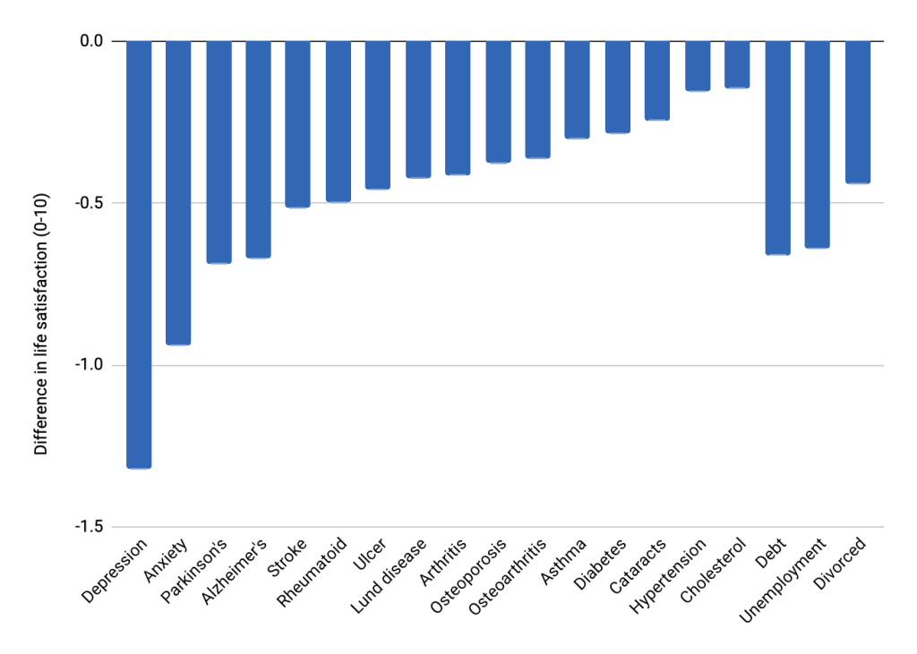
These mental health conditions are associated with greater declines in subjective wellbeing than many other health events (see Figure 1; HRI, 2020) or economic outcomes (such as income or unemployment; Clark et al., 2017). The burden of mental health suggested by wellbeing is relatively higher than that suggested by the DALYs (HRI, 2020, p.52). See Walker et al. (2021) for more discussion of mental health from a global priorities for wellbeing lens.
Figure 1: Difference in life satisfaction between persons with and without different conditions (reproduced from HRI, 2020)This is a reproduction of Figure 4.1 from HRI (2020). The description of how the effects were calculated is: “Context variables estimated using a single OLS linear regression controlling for gender, age, number of children, country, income, year, and remaining categories for marital status, education, and employment. Married used as the reference category for divorced. Bachelor’s degree used as the reference for no college (ISCED-3). Employed full-time used as the reference category for unemployed. Debt coded as dummy variable for negative or non-negative household net worth. Health status was also controlled for by adding additional control variables for all sixteen diseases except arthritis and asthma due to data limitations. Additional details in the online appendix.” (HRI, 2020, p. 50).
Yet despite their prevalence and severity, they receive little funding in low income countries. These disorders only receive ~1% of governmental health spending in LMICs“Low-income countries spend around 0·5% of their health budget onmental health services, lower-middle-income countries around 1.9%, upper-middle-income countries 2.4%, and high-income countries 5.1%.” (WHO | Mental Health ATLAS, 2017). (Vigo et al., 2019) and 0.3% of health-directed international assistance (Liese et al., 2019).
The low investment in mental healthcare shows. In LMICs, only 13.7% of people with mental illness receive treatment (Evans-Lack et al., 2018). This figure is 10.8% for anxiety, of which 2.3% is considered “potentially adequate” (Alonso et al., 2018), and 8% for depression (3% adequately treated; Moitra et al., 2022). Together, these facts suggest that improving mental health is a severely neglected problem.
1.2. Solution: psychotherapy is effective, cheap, and fundable
1.2.1 What is psychotherapy
Psychotherapy is a common treatment for depression (Cuijpers et al., 2020a; Kappelmann et al., 2020) and anxiety (Bandelow et al., 2017). Psychotherapy is a relatively broad class of interventions delivered by a trained individual who intends to directly and primarily benefit their patients’ mental health through discussion (Roth & Fonagy, 2006)Also activities and skill training (practising gratitude, improving social interactions, etc.).. Psychotherapies vary considerably in the strategies they employ to improve mental health, but some common types of psychotherapy are (Cuijpers et al., 2008): cognitive behavioural therapy (CBT), behavioural activation (BA), problem-solving therapy (PST), and interpersonal psychotherapy (IPT).
As we show in more detail in Section 1.2.2, meta-analyses of psychotherapy find that psychotherapy is effective at treating common mental health disorders. But how (and by which mechanisms) does psychotherapy lead to improved wellbeing (Beck, 2011; Cuijpers et al., 2019)? In general, it is thought that psychotherapy enhances wellbeing by addressing cognitive, emotional, and behavioural processes that contribute to psychological distress. Through therapeutic interventions, individuals may learn to modify maladaptive thought patterns, improve emotional regulation, and adopt healthier behaviours, which should contribute to reduced symptoms of anxiety and depression and increased overall wellbeing. However, while psychotherapy works, more causal evidence supporting specific mechanisms of how it works are needed (Lemmens et al., 2016, Cuijpers et al,. 2019, Janssen et al., 2021). One of the most supported causal mechanisms is that psychotherapy increases the number of days participants are able to work (Lund et al., 2024).
We think that psychoeducation might play an important role, especially in LICs. We think that general understanding about mental health problems is much lower in LICs, which is supported by the sparse provision of mental health treatment in LICs and some of the treatment provided can be actively harmful, such as putting people in chains (Walker et al., 2021; Moitra et al., 2022). Therefore, the first few sessions of a psychotherapy course could play an important psycho-educational role and thereby carry an important effect in a few sessions (or even one session) – more so than they would in high-income countries where we have relatively more awareness. If one has little understanding of why one is experiencing the terrible internal issues that come from depression or anxiety, or even attributes it to demons or curses, discovering that this is a treatable medical condition and that they are not on their own could be an immense source of relief. One of the authors (Michael Plant) conducted site visits (see Section 9.4) to both charities. He spoke to past and former clients, some of whom reported they had ‘no idea’ about mental health before. He also spoke to StrongMinds staff who mentioned that clients often think that poor mental health is due to being cursed.
There could also be unique mechanisms specific to the modality of psychotherapy. For example, in the context of group interpersonal psychotherapy (IPT) and problem-solving therapy (PST), two therapies we focus on in this report, have separate plausible mechanisms. For IPT, wellbeing may be improved particularly through the focus on interpersonal relationships. The goal of IPT is to help individuals identify and address problematic interpersonal dynamics, fostering better communication, conflict resolution, and social support within a group setting. This collective approach is thought to alleviate symptoms of depression and enhances participants’ social functioning and relational satisfaction, key determinants of well-being (Weissman et al., 2017). Meanwhile, PST is meant to target cognitive and behavioural pathways by teaching individuals systematic approaches to identifying and solving personal problems. The focus from the very first sessions is on setting out ways to solve the problems the client is experiencing. It is thought that, by enhancing problem-solving skills, PST increases individuals’ sense of self-efficacy and control over their lives, which leads to reductions in psychological distress and improvements in wellbeing (Nezu et al., 2012). Despite these potential differences, different forms of psychotherapy share many of the same strategies. Previous meta-analyses find limited evidence supporting the superiority of any one form of psychotherapy for treating depression (Cuijpers et al., 2020c; Cuijpers et al. 2021, Cuijpers et al. 2023). As such, we focus on psychotherapy as a class of interventions as a whole.
Note that psychotherapy is more than just a fallback option for when material interventions are lacking. By targeting maladaptive processes, psychotherapy is addressing root causes of mental distress, enabling people to overcome obstacles to their wellbeing that might otherwise persist. There is a bidirectional relationship between poverty and mental health: poverty causes low mental health, but low mental health also causes poverty (Ridley et al., 2020; see more on this topic in Appendix M1.3). Even in conditions of poverty, psychotherapy can be effective, just as those living in comfort are not immune to the impacts of depression and anxiety.
1.2.2 Effectiveness and other motivations
Extensive research has found that psychotherapy is effective at treating depression and anxiety. There has been a substantial amount of previous work to summarise and synthesise the effect of psychotherapy in high-income countries (HICs; Cuijpers et al., 2023). Meta-analyses have found moderate to large effects as indicated by standard deviation changes (Hedges’ g) in depression (Cuijpers et al., 2019, g = 0.72, RCTs = 309) and anxiety (Weitz et al., 2018, g = 0.52, RCTs = 52).
There are fewer works synthesising the effect of psychotherapy in LMICs. Singla et al. (2017, g = 0.49, RCTs = 29), Cuijpers et al. (2018, g = 0.73, RCTs = 36) and Tong et al. (2023, g = 1.10, RCTs = 105) are the most comprehensive and recent meta-analyses to synthesise the effect of psychotherapy on depression or anxiety in LMICsOther meta-analyses in LMICs focused on sub-populations or specific delivery mechanisms for mental health treatments. For example, Morina et al. (2017) focused on adult survivors of mass violence, Vallyand Abrahams (2016) only analysed the effects of peer delivered mental health treatment, and Purgato et al. (2018) focused on countries affected by humanitarian crises. Purgato et al. (2023), in a Cochrane review, focuses on community worker interventions for prevention. hAnrachtaigh et al. (2024) focused on task shifted and transdiagnostic approaches. . Note that Tong et al.’s (2023, Table S3) relatively high result reduces after removing outliers (g > 2, the same method we use) to 0.86 for upper-middle-income countries and 0.80 SDs for lower- and lower-middle-income countries.
Psychotherapy is often provided by highly-trained professionals, which can be too expensive and results in there being too few trained professionals to tackle mental health problems in LMICs. There are 1.6 mental health workers per 100,000 in LICs compared to 71.7 per 100,000 in HICs (45x times less; WHO, 2017, p. 31). Thankfully, psychotherapy can be more cheaply (but still effectively, albeit slightly less effectively) delivered with the use of lay practitioners – also called ‘task sharing’ and ‘task-shifting’ (Vally & Abrahams, 2016; Galvin & Byansi, 2020; Chowdhary et al., 2020; Karyotaki et al., 2022; Purgato et al., 2023).
Finally, our last motivation is that lay-delivered psychotherapy is a fundable and scalable way to address the problem.
1.2.3 Charities deploying psychotherapy
We previously ran a Mental Health Programme Evaluation Project (Donaldson & Grimes, 2021) to help us identify promising organisations based on the potential for effectiveness, low costs, and scalability. Of these, StrongMinds accepted to be evaluated and shared their data with us. As of Version 3, we added an evaluation of Friendship Bench because they accepted to be evaluated and shared their data with us. Both charities are scaling lay-delivered psychotherapy in Sub-Saharan Africa to hundreds of thousands of individuals each year. We note there are other similar charities we do not evaluate hereSee for example the other charities in the coalition for scaling mental health– which StrongMinds and Friendship Bench are part of – and Vida Plena..
Friendship Bench is a Zimbabwean based NGO that uses problem-solving therapy (PST) delivered by community health workers and peer deliverers trained by Friendship Bench to treat people with mild to moderate common mental health disorders (e.g., depression). In 2023, they reported that 220,766 individuals received at least one session of therapy through their programmes, 97% of these sessions were delivered through in-person counselling, the rest was via their Whatsapp programme (Friendship Bench Annual Report, 2023).
StrongMinds is an NGO that treats depression via lay delivered in-person group interpersonal therapy programmes (g-IPT; WHO, 2016), primarily in Uganda and Zambia. The lay deliverers are either community health workers or peers (who have gone through the programme themselves), who are first supervised by experts to deliver the programme. StrongMinds primarily delivers psychotherapy through partner governments and organisations where lay deliverers are trained to deliver g-IPT (78% of all clients; discussed in Section 8 and Appendix N); the remaining 22% of clients receive g-IPT by deliverers who are trained by StrongMinds staff.
See Table 9 in Section 5.2.1 for a comparison of the main differences between StrongMinds and Friendship Bench.
1.3 Evidence gap
If there were existing analyses of all the relevant data for Friendship Bench and StrongMinds that fitted our methodology, we could use these to calculate the cost-effectiveness. However, this is not the case so we had to gather all the sources of data and conduct the analyses ourselves. We explain the differences below.
There are previous meta-analyses of psychotherapy in LMICs (see Section 1.2), but psychotherapy meta-analyses do not always include follow-ups over time, and when they do, they bunch them in coarse categories (e.g., “follow-ups”, “0-6 months”, “6-12 months”). Instead, we ran our own meta-analysis where we extract all relevant follow-ups with granular continuous information about the follow-up time. This enables us to model effects over time in a continuous manner.
We also include a quantitative estimation of the household spillovers (the wellbeing benefits experienced by household members other than the direct recipient of psychotherapy).
To wit, neither of these analyses have been performed in previous academic studies.
We use monitoring and evaluating (M&E) pre-post data from the charities and apply an adjustment for the lack of a control group. As far as we know, no one has done this for the Friendship Bench and the StrongMinds data.
For each analysis we combine information from three sources of data, which we present in the next section.
2. Methodology
2.1 Sources of data and general flow
In this section we introduce the general flow and methods of our analysisWe have presented previous versions of this analysis in past reports (McGuire & Plant, 2021b; McGuire et al., 2022b; McGuire et al., 2023c). For a discussion of how this version differs from previous ones see the last citation and Appendix A. . For each charity, we have threeNote that charities also provide an additional extra source of evidence: their general M&E data, such as the number of people they treat in a year. We do not give a “weight” to this data, but we use the charity M&E information to inform other parts of our analysis. For example, we use information about attendance rates to determine the effect of dosage on the estimate of the effects and the number of people treated to determine the costs. sources of evidence we can use to estimate the effect of the programme (see Section 3 for more detail):
- General causal evidence (meta-analysis of RCTs of similar interventions in similar contexts). In this case, a meta-analysis of RCTs of psychotherapy in LMICs. This is generally higher quantity and quality evidence, and the lowest relevance.
- Charity-related causal evidence (RCTs of the charities’ programme, though not necessarily implemented by the charity themselves; we conduct a small meta-analysis if there is more than one effect size). This evidence is generally lower quality, most often because there are very few studies available. It is typically of medium relevance because while the RCTs are of the same programme (same training, curriculum, number of planned sessions, etc.), there are potential discrepancies that weaken the external validity (e.g., differences in actual sessions attended between RCTs and how the charity actually operates).
- Charity-related monitoring and evaluation (M&E) pre-post data (this data is generally collected by the charities themselves who survey participants before, after, and sometimes during, the programme). This evidence is generally lowest quality evidence (because it is not causal), yet it is the highest possible relevance. We include this source of data because of its high relevance.
Each of these sources presents a qualitatively distinct, but potentially informative, piece of evidence to draw upon.
Our analysis of each evidence source follows the same steps:
- We estimate the initial effect and duration in order to calculate the total effect for the recipient over time.
- We adjust the total effect to account for concerns about:
- internal validity (e.g., publication bias)
- external validity (e.g., the relevance of the evidence to how the programme is delivered in practice by the charity).
- We estimate the household spillover effectThe adjustments are multiplicative and the spillovers are based on a ratio, so whether we apply the adjustments first and then the spillovers or vice-versa does not change the results. to estimate the overall benefit for the household.
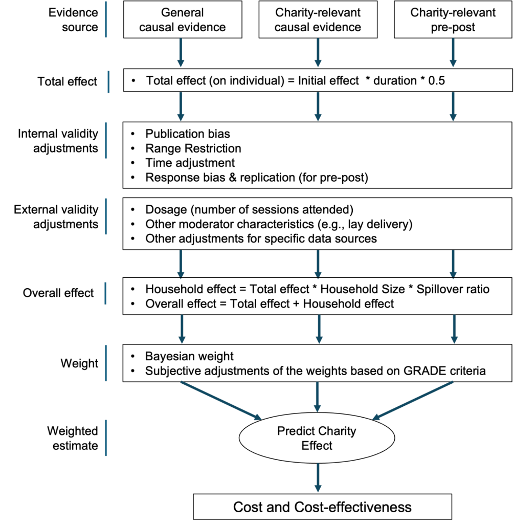
We then calculate our final, single effect estimate by combining the three estimates of the overall effect, using a mixture of Bayesian updating and subjective weights. We summarised the flow in Figure 2. We explain our methodology in more depth in the following subsections.
Figure 2: Flow of analysis.
We deviate from typical academic work in three regards. First, for most academic publications it is satisfactory to simply present the different versions of the analysis, we must decide to the best of our expertise which analysis to use for decision-making purposes. We want to make recommendations to, among others, donors who do not necessarily want to go through this analysis and choose their preferred specification. Second, we apply internal and external validity adjustments to the evidence in order to predict the effect in the context of the charity to the best of our ability. Third, we encounter other problems that have no clear academic precedent (e.g., weighting of different data sources). For all of these novel problems and decision points we provide our best-guess solutions. We also present how sensitive our results are to different solutions in our sensitivity analyses.
2.2 Effect
We estimate the effect on wellbeing of the intervention across all three data sources (see Section 4). For most of our evidence sources we use meta-analyses to combine the effects from different studies.
A meta-analysis, simply, is an average of standardised effect sizesWe standardised the effect sizes using standardised mean difference, first into Cohen’s d and then converted into Hedges’ g because it is a less biased estimate, especially for small sample sizes (Hedges & Olkin, 1985; Lakens, 2013; Harrer et al., 2021). This means that all the different results on different scales are converted into the same unit, standard deviations (SD). For more detail see Appendix B. (i.e., Hedges’ g; Hedges & Olkin, 1985; Lakens, 2013; see Appendix B). We use standard inverse-variance pooling of effect sizes (i.e., they are weighted by how precisely they are estimated). Note that we extracted multiple effect sizes from a study (every wellbeing outcomesWe also use affective mental health outcomes as explained in Section 2.2.3. These results are usually on negative scales (e.g., depression symptoms) where higher scores represent less wellbeing. In those cases we take the additive inverse (i.e., multiply by -1) so that every result is positively framed (increases mean increases in wellbeing). and every separate follow-ups). This means that there is dependency (i.e., non-independence) between the effect sizes within an intervention, which can overestimate the precision of the average effect if it is not accounted for. We deal with this by using multilevel meta-analysis models.
We followed the typical guidance for conducting meta-analyses from reference textbooks (Harrer et al., 2021) and Cochrane guidelines (Higgins et al., 2023) when it is available and pertinent. We conducted our analysis in R, primarily using the metafor package (Viechtbauer, 2010). There are many methodological paths to consider when performing a meta-analysis, which we discuss in Appendix C.
2.2.1 Total effect over time
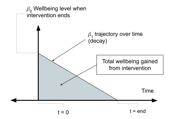
We are not just interested in the effect on the individual at the end of their treatment, but also the effect that the intervention has on them over time. To arrive at the total individual effects over time, we need to estimate two parameters: the effect post-intervention (the intercept in the model), and the change in the effect over time (the moderation by time)If the effect gets smaller over time, we call this ‘decay’. As we show in Section 4, we do find that effects decay over time.. Combining these two parameters generates a curve of the estimated benefits over time. The total benefit is the area under the curve from the time the treatment ends to until the effects become zero. We illustrate the total benefit in Figure 3 below.
Figure 3: Diagram of the total benefits of an intervention (psychotherapy)
To estimate the decay parameter we use a meta-regression that includes time since therapy endedIn this case the meta-regression would take the following form: g = β0+ β1(time)i +Xiβ + εi. Where: g is the standardised effect size, timeis the time since the intervention ended for study i, Xi is a vector of other control variables (Xi2,Xi3,…,Xik), β is the corresponding vector of other coefficients (β2,β3,…,βk), εi is the combined error term that encapsulates within and between study variability. . Meta-regressions are like regressions, except the data points (i.e., dependent variables) are effect sizes weighted according to their precision and the explanatory variables are study characteristics. Meta-regressions allow us to explore why effects might differ between studies.
We model the effect over time as linear as we do for most of our analyses (see our general methods page; stated simply, this means we assume the effect decays at a constant rate over time). To estimate the total effect for a recipient is then, for a linear coefficient, simply the area of the triangle applied to this context (area = ½ * base * height, where base = duration is the intercept divided by the decay coefficient, and height = intercept):
intercept * abs(intercept/decay) * 0.5
2.2.2 Overall household effect
Many interventions plausibly impact other members of the household in addition to the individual receiving treatment, a topic we motivated and discussed in McGuire et al. (2022). For this, we would ideally separately estimate the total effect for each distinct non-recipient household member directly then sum these effects with the effect of the recipient. However, there is so little data about spillovers that we need to use studies beyond those we directly use in our general meta-analysis to estimate it. We estimate this benefit as a function of the recipient benefit using a spillover ratio. The spillover ratio is the proportion of the recipient’s benefit that a non-recipient household member experiences.
S = spillover ratio = non-recipient household member effect / direct recipient effect
This spillover ratio, S, is then applied to every non-recipient household member to obtain the non-recipient household benefit, and added to the recipient benefit to arrive at the total household effect.
Non-recipient household benefit = recipient benefit * S * non-recipient household size
Which can then be combined with the direct recipient benefit (the total effect on the individual) to get the overall household benefit:
Overall household effect = recipient benefit + non-recipient household benefit
Note that in this report we will use the same household spillover across evidence sources since we only have data for the household spillover for psychotherapy in general, not for StrongMinds and Friendship Bench specifically.
2.2.3 Converting MHa and SWB SD-year changes to WELLBYs
In our analysis, we include multiple measures of subjective wellbeing (SWB) and affective mental health (MHa). Because these measures use scales of various lengths (e.g., 1 to 5, 0 to 100), we need to convert the effects to standard deviations (SDs) as is typically done in meta-analysisStandard deviations help us understand how spread out or different the scores are compared to the average score on a scale. No matter what scale is being used, one standard deviation (SD) means that, on average, the scores differ from the mean by a typical amount. For instance, on a 1-5 scale, one SD from the mean could be about 2 points. On a 0-100 scale, one SD could be around 20 points. In both cases, we are talking about one SD. By measuring effects in standard deviations, we can compare results across different scales, giving us a way to understand whether an impact is smaller, similar to, or larger than the usual amount of variation in the outcome.. The SD effects are then combined in a meta-analysis and then integrated over the years into a total effect. We want to convert this to wellbeing adjusted life-years (WELLBYs), where 1 WELLBY is the equivalent of a 1 point increase on a 0-10 wellbeing scale over a year (or equivalent).
To do so we follow our typical procedure (see the methods section of our website for more detail) where we multiply the effect in SD-years by our estimate of the typical SD on a 0-10 wellbeing scale. At the time of writing, this was an average SD of 2 points on the Cantril Ladder scale (based on the Gallup World Poll data: 1704 observations from 165 countries from 2005-2018 with a total sample of respondents of about 1,704,000).
|
Crucial consideration: by combining both MHa and SWB changes, this assumes they are both capturing similar constructs. Or, at the very least, that adding MHa measures does not overestimate our results. We argue that this is the case empirically and theoretically in a separate report (Dupret et al., 2024), see also Section 5.3. |
2.2.4 Confidence intervals
We present 95% percentile confidence intervals around our estimates. These are obtained by using the uncertainty generated in our models and then propagating it across the calculations (integral over time, adjustments, costs, etc.) using Monte Carlo simulations. This is how we can obtain a confidence interval around our cost-effectiveness estimates. See the methods section of our website for more detail.
2.3 Validity adjustments
By validity adjustment we refer to our attempt to correct for methodological inadequacies and make our estimates more reliable and generalizable to the charity specific context. These are discussed in Section 5.
Note that, for clarity, when discussing adjustments we refer to ‘adjustment’ as the factor one multiplies by, and ‘discounts’ as percent changes. For example, a 0.80 adjustment is a 1-0.80 = 20% discount.
2.3.1 Internal validity adjustments
Internal validity adjustments aim to provide more accurate estimates within the data analysed. This can be thought of as trying to predict what an estimate would be in perfect methodological conditions (e.g., large samples, replicated many times, absence of bias)Notably, this is leaving out other broader indicators of validity such as the intervention working as hypothesised and described, measuring the appropriate outcome, and the interpretation of the evidence corresponding with the evidence produced (Nosek et al., 2022).. One example of an internal validity adjustment we apply is to adjust the results of a meta-analysis for publication bias when it is identified.
2.3.2 External validity adjustments
External validity adjustments are meant to adjust for differences in the effect that arise from differences in the intervention, study type, population, or context compared to the implementation context of interest. The goal here is to estimate the effect of the interventions as they are implemented by the charities (not as by researchers in RCTs).
For example, we apply an adjustment because the number of therapy sessions attended differs between the causal evidence and the charity context. In several cases the deviations are substantial enough to require that we correct the results to better reflect the charity context.
We apply validity adjustments before we provide weights and aggregate our estimates across evidence sources. This is in order to reduce differences between the sources due to external validity as much as possible so that the weighting of data sources has to play a smaller role in accounting for external validity (thereby reducing the role of the most subjective part of our analysis). Note that even if we adjust for a factor (e.g., a deviation in relevance between the Baird et al. RCT and how StrongMinds operates today), this does not mean that we have fully accounted for its influence. Thereby, it can still play a role in our subjective weighting. This is because our adjustments cannot be perfectly calibrated.
2.4 Weights and aggregated estimate
For charities, we have three different types of evidence: General causal evidence, charity-related causal evidence, charity-related pre-post evidence. The relevance and quality of the different sources are summarised, coarsely, in Table 1.
Table 1: Relevance and quality of the different sources, coarsely summarised.
|
Quality |
Relevance |
|
|
General causal evidence |
High |
Low |
|
Charity-related causal evidence |
Medium |
Medium |
|
Charity-related pre-post data |
Low |
High |
For each charity we are trying to estimate its expected effectiveness in practice, and each of these sources presents a qualitatively distinct, but potentially informative, piece of evidence. We want to weight each source according to our relative confidence that it will improve our estimation of the charity’s true effect. We spent time searching the literature and pondering this issue but found almost nothing related to this problemThe best we could find was general literature about Bayesian concepts and methods such as shrinkage and Bayesian data fusion, which inform our general thinking but do not provide guidelines as to how to proceed with our particular issue.. We conclude that this is not a solved methodological problem and there are no clear guidelines we can refer to. Instead, we have to rely on our experience and methodological intuitions. We use a methodology that we think seems reasonable, given the evidence available (or lack thereof).
Our weights are averaged subjective weights from the research team. These are built from weights based on statistical uncertainty (quantified with Bayesian updating methods) and then adjusted subjectively to account for harder-to-quantify characteristics based on GRADE criteria such as ‘relevance’ (Schünemann et al., 2013). We relegate further discussion of the methods we used to Section 7 and Appendix L.
2.5 Cost and cost-effectiveness
Using information from the charities about their total expenses and number of clients treated we can calculate the cost per person treated. We use information from 2023, the latest year completed. We then calculate the cost-effectiveness of funding the charities.
2.6 Confidence
While we have reached the end of our quantitative parameters, we think it is important to try and contextualise the quantitative findings with an assessment of our confidence in the evidence and the estimates we base upon them (i.e., how confident we are that our analysis has produced the ‘true’ cost-effectiveness estimate of the charities). There are five factors that influence our confidence: depth of evaluation, quality of evidence (based on the GRADE criteria), robustness of the results to alternative analytical choices, site visits, and outstanding uncertainties.
2.6.1 Quality of evidence and GRADE
We explain our method for evaluating the quality of evidence here, because it is a primary consideration for our confidence, and explaining the methodology here will help clarify our view of the quality of the data sources as we present them.
We discuss our general approach to rating quality of evidence on our website, which is based on the GRADE criteria (Schünemann et al., 2013) with a few minor adjustments to make it a better fit for the charity evaluation context. GRADE is a widely-used, systematic tool for assessing evidence quality used across healthcare and research fields. Briefly, “quality of evidence reflects the extent to which we are confident that an estimate of the effect is correct” (Schünemann et al., 2013). Basically, this involves assessing how well the studies were designed and executed, if there was any risk of bias, the precision of the estimated effect (e.g., based on the number and size of the studies), how consistent results are (how heterogeneous), the relevance of the evidence, and whether there is any apparent tendency towards publication bias. To form a rating, we start with an initial rating based on ‘study design’: RCTs are ‘high quality’, while non-RCTs are ‘low quality’. Then, we adjust the initial rating as we go through the other criteria. Each of the other criteria are rated as either ‘no concerns’, ‘some concerns’, or ‘major concerns’. GRADE does not provide a mechanistic rating (i.e., it is not a mathematical calculation), but rather a method for making ratings in a systematic and transparent way. Note that our criteria for evidence quality are stringent, and we expect few, if any, interventions that we evaluate in LMICs will have more than ‘moderate’ quality evidence.
We provide a rough example of what the different quality of evidence ratings generally represent:
- High: To be rated as high, an evidence source would have multiple relevant, low risk of bias, high-powered RCTs that consistently demonstrate effectiveness and have little to no signs of publication bias.
- Moderate: If the evidence source moderately deviates on some of the criteria above, it would be downgraded to moderate. For example, it would be moderate if it has some moderate issues of risk of bias, publication evidence from a single well-conducted RCT, or evidence from multiple well-designed but non-randomised studies that consistently demonstrate effectiveness.
- Low: If the evidence deviates more severely on these criteria it could be downgraded to low. For example, it would be low if it does not use causal studies (pre-post, correlations, etc.).
- Very low: If the evidence deviates even more severely on these criteria, or is low on many criteria, it can be downgraded to very low.
The GRADE method is not formulaic, but instead offers a structure for making these assessments, so these examples above should be viewed as heuristics rather than strict criteria. We evaluate the different sources of evidence on their quality of evidence and then combine them together. Ideally, we would combine ratings in a proportionally and quantitative manner; the principle would be that if the evidence quality for one source (e.g., the charity-related RCTs) is different from the rest and it contributes to 50% of our final estimate, then our overall rating should reflect that. However, it is difficult to convert these qualitative factors into quantitative ones. Therefore, we follow this principle but we ultimately rely on some subjective fuzzy combination.
We present our quality of evidence ratings at the end of each data source in Section 3, bring them together for a summary and overall rating in Section 9.2, and provide more extensive detail in Appendix J.
3. Data
We already gave a coarse overview of the different types of evidence we used in Table 1. In Table 2 we provide a more detailed summary of the evidence. Throughout this section we go on to explain the sources of the evidence, any alterations to the data, and our confidence in its quality.
Table 2: Characteristics of evidence sources.

Note. Friendship Bench (FB) and StrongMinds (SM).
3.1 General meta-analysis evidence for psychotherapy in LMICs
The general evidence we use stems from a systematic review and meta-analysis we conducted of all RCTs of psychotherapy’s effects on subjective wellbeing, depression, anxiety, or distress in LMICs. We focus on LMICs rather than LICs or Sub-Saharan Africa (where Friendship Bench and StrongMinds operate) because we wanted a wider understanding of psychotherapy in places other than HIC and because it can serve as a ‘prior’ understanding for more mental health charities in the future which might operate in a different part of the world but still be in LMICs.
We discuss the methodology for this systematic review, effect size extraction, references, and present forest plots in Appendix B. We aimed to perform the systematic review in line with standard guidelines (e.g., Cochrane) to a degree that would be acceptable for a top academic journal (which we plan to submit the meta-analysis to)For instance, we included double checking of our extracted data with two double-checkers who were not the initial extractors who checked every number we had extracted (this is the method used for our meta-analysis of cash transfers published in Nature Human Behaviour; McGuire et al., 2022a). This also included doing two rounds of risk of bias analysis to check for and resolve potential mismatches in evaluations..
In sum, we have found and extracted results for 127 papers. However, not every paper corresponds to one intervention, as sometimes different papers report on the same intervention (for different follow-ups, for example) or a paper might report on two interventions (see footnote for more detailBasset al. (2006) is a follow-up of Bolton et al. (2003). Fard et al.’s (2018) sample was split between those who did a pre-test at baseline and those who did not. Namasaba et al. (2022) reported on one intervention for caregivers of children with disability in the home, and one intervention for caregivers of children with disability in schools. The Health Activity Program was reported on by multiple papers (Patel et al., 2017; Weobong et al., 2017; Bhat et al., 2022). The Thinking Healthy Programme Peer-Delivered (THPP) in India was reported on by multiple papers (Fuhr et al., 2019; Bhat et al., 2022). The Buenaventura and Quibdo interventions were both reported on in multiple papers by Bonnilla-Escobar et al. (2018, 2023a, 2023b). Weiss et al. (2015) reported both a CETA and a CPT intervention.). Our analysis includes 127 interventions, but note that, henceforth, by ‘study’ we will mean ‘intervention’ and not ‘paper’.
For many interventions we extracted more than one effect size, because the intervention had multiple outcomes that fit our inclusion criteria and multiple follow-ups. This resulted in k = 127 interventions with m = 361 effect sizes, with O = 83,867 observations from N = 31,914 unique participants.
We made two important restrictions to this initial dataset for our use in the cost-effectiveness analysis (explained in the following subsections).
- We removed studies assessed overall as having ‘high’ Risk of Bias (RoB; Sterne et al., 2019). See Section 3.1.1 below.
- We classified (and removed) effect sizes larger than 2 standard deviation (SD) changes as outliers. See Section 3.1.2 below.
|
Crucial consideration: In our sensitivity analysis we present alternative analyses where we did not remove outliers and high risk of bias studies in Section 9.3.4. For most academic publications, it is satisfactory to present all the different possible analyses and their results without having to pick one. However, we must also decide on what is the best analysis because we are making an evaluation to inform decision making. Overall, we think that removing high risk of bias studies and outliers is the right analysis decision and increases the accuracy and validity of our results. This is also the more conservative choice. See Appendix P for more detail. |
3.1.1 Risk of Bias analysis
We conducted a Risk of Bias (RoB; Sterne et al., 2019) analysis (with a second round to check for and resolve potential mismatches in evaluations). For more detail, see Appendices B and P4. This is the academically standard way of assessing if a study has flaws in its design or implementation which could ‘bias’ the result (downward or, more commonly, upwards). Assessing RoB is a sort of ‘due diligence’ for a systematic review and meta-analysis, one that is time consuming (but often, although not always, done for academic publications). A classic example of bias in a medical trial would be participants not being ‘blinded’ as to whether they receive the drug or a placebo.
Raters assess studies on five subdomains according to criteria set out by Cochrane (Sterne et al., 2019). For a study to be considered ‘low’ risk of bias, all five domains need to be rated as low. If at least one of the criteria is evaluated as ‘some concerns’, then the overall rating will be ‘some concerns’. If at least one of the criteria is evaluated as ‘high’ risk of bias, then the overall rating will be ‘high’. See Table 3 for the results.
Table 3: Risk of Bias distribution before any removals.
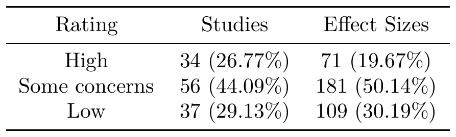
Readers unfamiliar with RoB analysis should not assume that a ‘high’ risk of bias indicates that the study’s author(s) are corrupt or incompetent, only that they are reasons to doubt the results. Note that it may be difficult to conduct some studies in less biased ways depending on their context. In our case, we assumed studies with high risk of bias are not as reliable and are likely to inflate the effect estimate. Hence, of our 127 interventions, we exclude 34 interventions (or 71 effect sizes) with ‘high’ risk of bias. Leaving us with 56 interventions rated as ‘some concern’ and 37 interventions with ‘low’ risk of bias (for a total of 93 interventions). See Section 9.3.4 and Appendix P for how much this influences the analysis (not much).
|
Crucial consideration: We considered having our analysis run purely on ‘low’ risk of bias RCTs but we decided against it for the following reasons: this loses a lot of information, not all our moderators of interest (as per Appendix G2) can be well run, a study can be considered at more risk than ‘low’ as long as one subdomain is not considered ‘low’ risk (which could be stringent), the results are not very sensitive to this type of analysis, and cash transfers (our typical comparison point) do not have low risk of bias studies. See Appendix P4 for more detail. |
3.1.2 Outliers
In the literature, there are many approaches to determining outliers, but no specific set recommended method, especially not for our kind of meta-analysis that uses follow-ups. Based on visual inspection, there are clearly large implausible effect sizes in our data (up to ~10 SDs) that we would consider outliers. These results seem implausible and potentially due to poor study quality or statistical noise (e.g., stemming from small samples). See Figure 4 for an illustration.
Figure 4: Histogram of effect sizes, showing how many count as outliers.
We removed outliers, which we define as effect sizes with values above 2 SDs (g > 2 SDs). This threshold is consistent with other meta-analyses (Cuijpers et al., 2018; Cuijpers et al., 2020c) including the clearest precedent to our own (Tong et al., 2023).
|
Crucial consideration: We tried other thresholds and methods and found that overall our choice of (g > 2 SDs) is consistent with the results of most other methods (and conservative among them). We think that removing outliers is the right choice for this analysis, and conservative (the cost-effectiveness increases if we include them). See Appendix P3 for more detail. |
This meant removing 40 effect sizes. An extra 15 effect sizes that would have been outliers had already been removed because they were evaluated as ‘high’ risk of biasOutliers can emerge for various reasons unrelated to risk of bias. For example, studies with smaller sample sizes (which are not marked as ‘high’ risk of bias) are more prone to variability, which can lead to exaggerated effect sizes. . Overall, this led to the removal of 9 studies beyond those removed for risk of bias. This might sound like a lot but remember that we have over 100 studies, in which we extract multiple effect sizes. Most other meta-analyses tend to have fewer studies and only extract one or two effect sizes per study.
3.1.3 Overall data after removals
This leaves us with k = 84 interventions and m = 250 effect sizes with O = 68,443 observations from N = 25,363 unique participants. Of these studies, 48 (57%) are rated as ‘some concerns’ and 36 (43%) of these studies are rated as ‘low’ risk of bias. The mean sample per effect size was N = 274 (median = 129, range 19 to 7,330). The mean follow-up time was 0.28 years (median = 0.10, range 0 to 4.87) or 0.39 years (median = 0.18, range 0 to 4.87) for the latest follow-up of each study. On average, studies had 2 follow-ups (one post treatment and one later on; range 1 to 4) with 39 (46%) of studies having more than one follow-up. On average, studies had 2 different outcomes (range 1 to 4) with 52 (65%) of studies having more than one outcome. This data is illustrated in Figure 5.
Figure 5: General meta-analysis effect sizes.
Note. The colours represent different combinations of interventions and outcomes and their potential multiple effects over time (linked by a line to show their trajectory over time).
We assess the overall quality of evidence of the general causal evidence to be ‘moderate’ overall, based on our stringent GRADE-adapted criteria (explained in Section 2.6.1). The evidence base includes a large number of RCTs, with decently precise estimated effects, and limited risk of bias. However, there is some inconsistency in the effect sizes (measured as heterogeneity), and the studies are not directly related to the contexts of the charities. There is also substantial publication bias that — while adjusted for — may still bias the results.
3.2 Charity-related causal evidence
3.2.1 Friendship Bench causal evidence
From a search of the meta-analytic data and asking the charity, we find and use four RCTs (k = 4 studies, m = 15 effect sizes, N = 2011 unique participants, O = 7377 observations) studying the effect of problem solving therapy (PST) delivered by Friendship Bench specifically (not PST generally): Chibanda et al. (2016, m = 3, N = 573, O = 1563), Haas et al. (2023, m = 8, N = 516, O = 4128), Simms et al. (2022; m = 2, N = 842, O = 1530), and Bengtson et al. (2023, m = 2, N = 80, O = 156). See Figure 6 for a detail of the effect sizes over time.
Figure 6: Friendship Bench effect sizes.
Note. The colours represent different combinations of interventions and outcomes and their potential multiple effects over time (linked by a line to show their trajectory over time).
The results reported by Chibanda et al. (2016) are at the cluster level, which is not the structure of results we look for in such meta-analyses and would suggest problematically large effect sizes (above 3 SDs). We contacted the authors and they provided individual level results for us with the adjustment for clustering.
While we use standard criteria for including studies in the general evidence (i.e., inclusion criteria for the systematic review, remove outliers, and remove ‘high’ risk of bias studies), we assess the relevance and quality of charity-related studies on a case by case basis, because there are fewer studies, they receive more weight, and we expect this will lead to more accurate results.
Two of the RCTs we included do not fit our pre-stated inclusion criteria as established in our protocol (McGuire et al. 2024). In Bengtson et al. (2023), the intervention was provided over the phone, rather than face to face, because of Covid-19. In Simms et al. (2022), the intervention was provided to adolescents rather than adults. We ran a robustness check where we compare the models with and without these studies (see Table 6 of Section 4.2.1). Adding these studies does not change the results much, it mainly increases precision and reduces heterogeneity. Furthermore, in terms of the total effect, adding these studies is more conservative.
In our risk of bias assessment, we evaluated Haas et al. (2023) and Bengtson et al. (2023) as ‘some concerns’. We rated Chibanda et al. (2016) and Simms et al. (2022) as ‘high’ risk. We will now provide context for this rating. First, remember that ‘high’ risk of bias does not mean that authors conducted their study in a corrupt or incompetent, only that elements of the study could make us doubt the results. Also, it suffices that only one ROB subdomain (as is the case for both these studies) to be rated as ‘high’ for the study to be rated as ‘high’ ROB overall.
In most psychotherapy studies, patients know (i.e., they are not blinded) they are receiving psychotherapy (it is not easy to placebo psychotherapy), but this does not automatically lead to a ‘high’ risk of bias evaluation (Sterne et al., 2019). Simms et al. (2022) was rated as ‘high’ risk of bias because there was no ‘allocation concealment’: while the allocation to the groups was randomised, the sequence by which participants are allocated into the control or treatment group was not hidden (i.e., not blinded). Simms et al. do not provide more details (and the trial pre-registration only mentioned that the “allocation was determined by the holder of the sequence who is situated off site”), so we cannot be sure how this affected the results. However, the Risk of Bias tool considers this a ‘high’ risk because without this blinding to the sequence, staff (or participants) might have known which group someone would be placed in, which could lead to selection bias, where people could – on purpose or by accident – affect who goes into which group, making the groups less balancedIn the detailed guidelines,RoB authors mention this possibility: “Even when the allocation sequence is generated appropriately, knowledge of the next assignment can enable selective enrolment of participants on the basis of prognostic factors. Participants who would have been assigned to an intervention deemed to be inappropriate may be rejected, or participants may be directed to the ‘appropriate’ intervention, for example by delaying their entry into the trial until the desired allocation appears. For this reason, successful allocation sequence concealment is an essential part of randomization.” (p. 11).. Other than for that criterion, Simms et al. would be considered ‘some concerns’. As shown in the model in Table 6 of Section 4.2.1, not including Simms et al. does not affect the modelling much; it is actually more conservative to include Simms et al. (total effect excluding: 1.12 SD-years; total effect including: 0.86 SD-years).
Chibanda et al. (2016) was rated as ‘high’ risk of bias because some participants received external treatment and it was not balanced between the control and treatment group: “At follow-up, 8.1% of control group participants and 5.4% of intervention group participants reported receiving counseling in the previous 6 months, and 11.1% of control group participants and 7.7% of intervention group participants reported visiting a spiritual healer. Fifteen participants in the intervention group and 34 in the control group were referred to tertiary care and prescribed fluoxetine." (p. 2622). Removing Chibanda would reduce the effect (see Table 6 of Section 4.2.1), but we do not think we should remove it for the following reasons:
- This is the most relevant RCT of Friendship Bench and so we think we should take it into account.
- The imbalance in external treatment is due to the control group receiving more external treatment, which would suggest a downward (rather than upward) bias in the effect estimate.
- Other than for this point, Chibanda et al. would only be considered ‘some concern' based on the other domains from the risk of bias evaluation.
- If we remove both Chibanda et al. and Simms et al., the overall cost-effectiveness of Friendship Bench (based on our weighting of the three sources of evidence) is still high at 37 WBp1kIf one put a 100% of the weight on the Friendship Bench RCTs (instead of splitting the weights across different sources) and removed Chibanda et al. and Simms et al. the cost effectiveness would be lower, at 15 WBp1k, but still 2 times the cost-effectiveness of cash transfers..
Thus, we think the rating of ‘high’ ROB is not concerning in this case, and due to the relevance of the study to FB, it provides valuable information that we want to include.
We assess the overall quality of evidence of the Friendship Bench RCT evidence to be ‘low to moderate’, based on our stringent GRADE-adapted criteria (explained in Section 2.6.1). While there are only a small number of studies (k = 4), the sample size is decent, the studies are mostly relevant, the imprecision and inconsistency are moderate, and we have relatively little concern about publication bias. The biggest concern is about risk of bias.
3.2.2 StrongMinds causal evidence
There is one RCT that we consider as ‘charity-related’ evidence for StrongMinds: Baird et al. (2024; k = 1 study, m = 6 effect sizes, N = 1896 unique participants, O = 7125 observations). This has been published as a working paper and not (yet) in a peer-reviewed journal. We discuss the structure and data from the trial, next. Then, we explain why we think this study is less relevant than it might seem at first.
In Version 3, we had only seen a preliminary results table (but not the report). We were not permitted to directly use these results so we used a placeholder low result instead. Now that the report is out, we can use the full results and comment on the full extent of the relevance of the study.
This RCT evaluated a pilot program implemented by BRAC with training and support from StrongMinds. The intervention was a 14-week group interpersonal therapy (g-IPT) delivered by peer facilitators to adolescents in Uganda. Participants were divided into three groups: a control group, a group receiving only g-IPT, and a group receiving g-IPT along with a one-time unconditional cash transfer of $69 provided immediately after the first follow-up (g-IPT+). There were three follow-ups: one after the end of the intervention, one about one year after the intervention (by which point COVID had struck), and one about two and a half years after the intervention.
We extracted results and calculated effect sizes for all three follow-ups, on the GHQ-12 and PHQ-8 scales (see Figure 7). At the first follow-up, Baird et al. combined the results of the g-IPT and g-IPT+ groups, because the cash transfer had not yet been announced to the g-IPT+ group, meaning their treatment was identical to the g-IPT group up to that point. For the subsequent follow-ups, the g-IPT and g-IPT+ groups were evaluated separately.
Figure 7: Baird et al. effect sizes.
Note. The colours represent different outcome scales and their multiple effects over time (linked by a line to show their trajectory over time).
These six effect sizes are very small and their confidence intervals cross zero, except for the first follow-up, on the GHQ-12 (a measure of general mental distress).
The results of this RCT have been highly anticipated because – at face value – it is the most relevant causal evidence of the impact of StrongMinds. We include this study as ‘charity-relevant’ evidence because it implemented a version of StrongMind’s lay-delivered group IPT, and it took place in Uganda. However, there are many important limitations to the relevance of this study to how StrongMinds operates in practice today, and it should be understood that this RCT was not a direct evaluation of StrongMind’s own core programme.
We explain these limitations in depth in Appendix L3, but we summarise them below for brevity. We strongly encourage interested readers to review this appendix for our full rationale.
The Baird et al. RCT has limited relevance because:
- It was a pilot: The
RCT was a pilot from 2019 of the first time StrongMinds had implemented their programme via
a partner organisation, the first time they had worked with adolescents, and the first time
they had used youth facilitators. StrongMinds has noted important lessons learned from the
pilot, and has since made substantial changes to its work, especially
with partners and with adolescentsAmong other changes, StrongMinds (2024) mentions that “After the BRAC partnership, StrongMinds hired a human-centered design firm, which studied the entire adolescent program from a user perspective. This led to multiple changes in the program, including: the implementation of emotion cards and other visual aids to assist different types of learners; the introduction of icebreakers to create comfortable atmospheres; and the use of journaling to help engage clients. We determined that IPT-G-trained teachers and Village Health Technicians (part of the VCT) were more effective in facilitating adolescent therapy groups than youth.”
So, StrongMinds is no longer using ‘youth’ peers from the community for treating adolescents (only 18% of StrongMinds’ clients) in the same way as was used in Baird et al. Instead, facilitators for adolescents are either g-IPT trained teachers, community health workers, or community members who have graduated from a programme of StrongMinds treatment for their own mental health problems.While it is possible that some of these facilitators are between 19-22 years old, we expect this will be a small proportion, and they would need to have prior experience delivering community services and they would have gone through additional training with StrongMinds.
(StrongMinds, 2024; Baird et al., 2024). - Different population: The RCT treated adolescents, while StrongMinds mainly treats adults (82% of the time).
- Different delivery: The RCT used young and inexperienced peer facilitators (aged 19-22), while StrongMinds uses adult facilitators with prior experience delivering community services. The RCT facilitators were also newly recruited and were delivering psychotherapy for the first time, while StrongMinds trains facilitators today over at least twelve sessions before allowing them to lead sessions independently.
- Worse implementation: The way the program in Baird et al. (2024) was implemented differed from StrongMinds’ current model.
- Less compliance: 44% of participants in Baird et al. (2024) failed to attend any sessions, compared to only 4% of clients completing 0 sessions with StrongMinds after being referred to take part in its programmeWhile 44% failing to attend any sessions could still be a high compliance rate for astudy with participants recruited from the community, the difference in compliance rates compared to StrongMinds underscores that the population and/or programme implementation in the RCT were substantially different from that of StrongMinds in general. .
- Different attendance: Participants in Baird et al. (2024) who attended at least one session attended an average of 10.56/14 = 75% sessions in total. StrongMinds clients attend an average of 5.63/6 = 94% sessions.
- Limited supervision: StrongMinds have communicated to us that there were constraining factors that meant they could not be as involved as they would be with partners. Notably, they told us that, to accommodate the school schedules of many clients, group therapy sessions were hosted on weekends, which limited StrongMinds’ ability to supervise and provide feedback to the BRAC facilitators since their employees worked during the normal work week.
- COVID-19: the long-term data collection occurred soon after the onset of the pandemic, which of course had profound effects on society and may have had unexpected impacts on the study. As a notable example, the group receiving cash transfers reported significant negative long-term effects on wellbeing. This is a surprising result given the robust effect of cash transfers on wellbeing (McGuire et al., 2022a), and suggests that the unique circumstances of the pandemic may have undermined the effectiveness of the interventions. In the same way this study would not update us strongly about the impact of cash transfers generally, we do not think it updates us strongly about psychotherapy.
So, despite taking place in Uganda and using a version of StrongMinds’ model, this study was meaningfully different in important ways from StrongMinds’ own, current programme (it was a pilot programme with a different population, different delivery, worse implementation, and it took place during COVID-19).
|
Crucial consideration: Because of these limitations in the relevance of the Baird et al. (2024) study, we give this study less weight in our analysis than we would otherwise (See Section 7.3 for more detail). |
We assess the overall quality of evidence of the StrongMinds RCT evidence to be ‘low’, based on our stringent GRADE-adapted criteria (explained in Section 2.6.1). There is only one RCT (Baird et al., 2024), which means we are unable to assess inconsistency. While it has a decent sample size and was pre-registered so we are less concerned about publication bias, its relevance to StrongMinds’ current program is potentially limited.
In our risk of bias assessment, we evaluated Baird et al. (2024) as ‘some concerns’ because of its low levels of compliance (44% of participants failed to attend any sessions). Baird et al. explore the effect of compliance using a LATE analysis (see Section 5.2.4), but the ROB criteria still considers this to lead to ‘some concerns’. On the other subdomains we evaluated Baird et al. to be ‘low’ risk of bias.
3.2.2.1 Other StrongMinds-related data
Note there are other pieces of data from StrongMinds to be considered (see also Section 3.3.2 for the M&E pre-post data):
- There is a controlled (but not randomised) study of StrongMinds’s programme in Uganda on adult women (N = 371; Peterson et al., 2024). The participants were assigned to treatment or control groups based on their community of residence. We do not directly include this study in our analysis because participants were not randomly assigned to the different groups and therefore this is not an RCT. However, this could be considered highly relevant. We present the results in 4.2.2.
- StrongMinds has run a non-superiority (A/B) trial comparing the effects of shortening their course to 6 sessions from 8 and sorting the groups based on the types of depression triggers the clients have. While this is an RCT, it is comparing two groups receiving treatment from StrongMinds, so we are not able to use it directly. However, when information about the trial will be published, we will use it as a sensibility check for both the pre-post in Baird et al. (2024) and the M&E pre-post results StrongMinds report.
3.3 Charity-related pre-post
We now turn to a discussion of the internal monitoring and evaluation (M&E) pre-post data the two organisations collected for their own purposes. The charities often report some general results from this M&E pre-post data in their annual report. However, they have kindly given us access to more detailed data for us to use in our analysis. This data being private, we only present aggregate results.
3.3.1 Friendship Bench
The 2023 pre-post data from Friendship Bench is a relatively small M&E sample size (at least compared to StrongMinds; see Section 3.3.2) and from a low response rate, so we ultimately only give a limited amount of weight to this source of evidence. The data comes from 3,433 clients, which is only a 20% response rate of the 17,463 clients who were sampled to be contacted at a 6 week follow-up survey to complete the SSQ-14 (2023 annual report)The annual report mentions 3,326 clients rather than the 3,433 in the data Friendship Bench has provided us. This difference comes from data Friendship Bench might have received or processed later in the year..
Friendship Bench shared with us the results from this survey. There is an average reduction in symptoms of -4.13 points on the SSQ-14 (a 14 point scale). Friendship Bench have also shared with us data covering the whole of 2021-2024, which has a similar reduction in symptoms of -4.18 points on the SSQ-14. We use the 2023 data because it is the latest complete year and the most relevant for our purposes.
We are unsure how informative these results are. Still, we think it is worth noting that some of these estimates are much lower than our other estimates for Friendship Bench’s effects. Hence, including, and giving weight to, the Friendship Bench M&E pre-post results decreases the overall cost-effectiveness of Friendship Bench, acting as a more conservative part of our analysis.
We assess the overall quality of evidence of the Friendship Bench pre-post evidence to be ‘very low’, based on our stringent GRADE-adapted criteria (explained in Section 2.6.1). The primary reason is that we do not have a true control group, and our method to deal with this is limited. There is also the potential for substantial risks of bias.
3.3.2 StrongMinds
StrongMinds aims to collect M&E pre-post data from every client. StrongMinds shared with us the pre-post data for clients in Uganda and Zambia in 2023 (N = 240,182; 231,473 of which attended at least 1 session). 218,045 clients provided results post treatment (91% response rate). This is a very large sample and representative of StrongMinds because it involves almost allThey did not include results from the 8,199 (3.4%) clients from countries outside of Uganda and Zambia (e.g., Kenya) because obtaining data from those partners requires significantly more effort to request and integrate. the clients treated in 2023 (239,672 clients attended at least one session). The average reduction in symptoms of -13.04 points on the PHQ-9 (27 points scale) – a very large reduction.
We assess the overall quality of evidence of the StrongMinds M&E pre-post evidence to be ‘very low’, based on our stringent GRADE-adapted criteria (explained in Section 2.6.1). The primary reason, as for Friendship Bench, is that we do not have a true control group, and our method to deal with this is limited. There is also the potential for substantial risks of bias, which seems more likely given that the effects of the M&E based estimate is much higher than the other sources of evidence.
4. Total recipient effect
In this section we discuss the total effect on the individual for each source of evidence. This is summarised in Table 4.
Table 4: Summary of the total recipient effect by evidence source
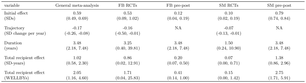
Note. Friendship Bench (FB) and StrongMinds (SM). The parentheses represent 95% confidence intervals.
4.1 General meta-analysis evidence for psychotherapy in LMICs
To estimate the total effects of psychotherapy for its direct recipient, we estimate the initial effect of psychotherapy and how long these effects last using the moderating effect of time. Taking these two together, we can calculate the total recipient effect.
However, we make two adjustments in our modelling that decreases the total effect we generally expect of psychotherapy:
- There are a few very longterm follow-ups (4 effect sizes) who exert a lot of influence on the total effect. Readers can see in Table 5 that the duration and total effect is much larger in the model that includes these effect sizes (‘with longterm follow-ups’) than in the model that does not (‘time’). We could not find clear direct precedent on what to do, and we did not think we should completely ignore their influence. So we exclude these follow-ups from our modelling but we created and applied a time adjustment factor (see Section 5) that increases the total effect in a way that takes some (but not all) of the influence of the very longterm follow-ups. See Appendix D1 for more details.
|
Crucial consideration: We could not find a clear precedent method for dealing with the high – but not clearly undue – influence of the long-term follow-ups. We present the influence of this decision point in our robustness checks (see Section 9.3) and explore this issue more in Appendix D1. We considered the potential role of attrition, publication bias, how the importance of psychoeducation could explain longterm results, and other psychotherapy studies showing longterm results. We conclude that these longterm effect sizes should be given some weight. Ultimately, we give the total effect with the longterm follow-ups about 50% of the weight compared to the model without them, instead of taking the model with them at face value. This involves taking the model without the longterm follow-ups but increasing its total effect with an adjustment of (1.15 * 0.5 + 2.40 * 0.5)/1.15 = 1.54 to its total effect. This can be seen as conservative. |
- We adjust for the biasing effects from the large share (23%) of studies in our sample that were conducted in Iran. In the ‘core model’ of Table 5 the ‘Studies in Iran’ predictor shows that a study from Iran will on average have larger effects than other studiesNote that we are just referring to the intercept. The Iranian studies do not show unusual effects over time (see Appendix D).. We cannot think of a plausible explanation and infer there is bias and this indicates an overestimateDuring our first extraction we had internally noted that many of these RCTs appeared to be of questionable quality for reasons outside of those captured by RoB (e.g., underpowered sample sizes, typos, poor formatting, inconsistent reporting of figures). Furthermore, Iran has been identified as one of the countries with issues of fake academic papers (Else & Van Noorden, 2021; Richardson et al., 2024). We are not saying these are fake studies, just that this is an additional reason for our scepticism. Overall, it seems unreasonable to take these at face value. However, we do not have strong reason to directly remove these studies (they are not necessarily outliers or ‘high’ risk of bias studies). Instead, we use as our core model a model that controls for this bias by including Iran as a predictor, and we use the smaller intercept this model predicts. See Appendix D2 for more details.
These models are summarised in Table 5 and the integral over time is illustrated in Figure 8. The parameter for time is a continuous variable where we extracted the time after the end of the intervention for each effect size. This is a continuous relationship (i.e., the change in SD for each year of follow-up time). The parameter for studies from Iran is a binary of whether the study is from Iran or not. This represents how much higher the results from Iranian studies are. Duration is the number of years until the effect reaches zero, and total effect is the integral of this effect over the years (see Section 2.2.1). Note that we are briefly summarising this modelling. Interested readers should consult Appendix D.
Table 5: Primary moderators for general evidence of psychotherapy.
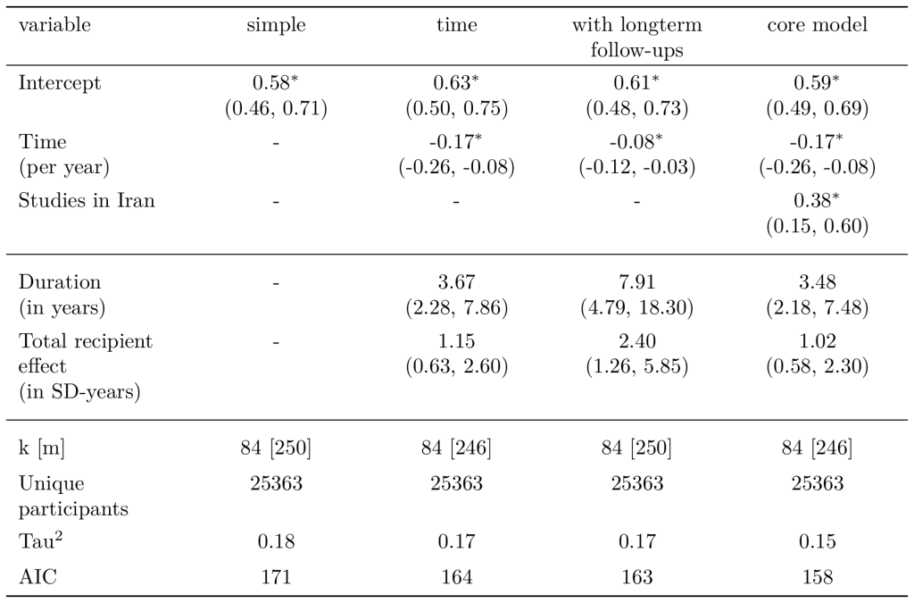
Note. All the effects presented above the first separation line are coefficients from the meta-analysis model. Their effects are in Hedge’s g (SD changes). The parentheses represent 95% confidence intervals. Statistical significance is represented such that * p < 0.05; ** p < 0.01; *** p < 0.001.
Figure 8: Illustration of the integral for the general meta-analysis of psychotherapy.
Note. The blue line represents the average trajectory over time (from post-intervention to when it reaches zero) according to the model without the extreme follow-ups and the red line represents that of the model with the extreme follow-ups. The respective shaded areas represent the integrated effect over time, the total recipient effect.
4.1.1 The general evidence as the ‘prior’ for the charities
We refer to the ‘general evidence’, or ‘general meta-analysis’, or ‘general prior’, interchangeably. These all refer to this general meta-analysis of psychotherapy in LMICs. Our ‘core model’ from our meta-analysis of psychotherapy studies in LMICs (the one moderated by time and controlling for Iran) serves as the ‘prior’ and source of evidence for the charities.
In a broad sense, the general evidence tells us what to expect of psychotherapy in a LMIC as delivered by the charities before we see more data about the charities. Hence, it provides a prior that psychotherapy charities might be effective. We then also look at charity-related data to form a view about the specific charities. If charity-related data is much more or much less effective than the general evidence, it would be somewhat surprising and worth investigating the discrepancy. It may be explained by one data source being more relevant and accurate, or that there are quality issues with one of the data sources.
For both StrongMinds and Friendship Bench we use the general evidence as a source of evidenceIn our previous analyses we estimated two different general effects of psychotherapy, one for each charity. This is because to estimate the effect based on the general evidence (which we referred to as the “prior”), we removed the charity relevant studies from the general psychotherapy datasets (namely, we removed the Friendship Bench RCTs) so that we would not be double counting. This makes theoretical sense when we were doing the formal Bayesian analysis because you do not want the same information entering into the prior and the evidence that updates the prior. However, this also led to a headache in reporting since it meant that we had slightly different figures for the parameters like the average initial effect, decay rate, duration, and publication bias but also slightly different figures for every moderator model. It might confuse the reader. Furthermore, this is a computing headache because it triples the computing time for the analysis. We decided that in this version of the analysis, the conceptual elegance is not worth the effort. So all estimates of the charity effects based on the general evidence will start from the same average effects which we will then adjust according to moderator analyses and validity adjustments to make it a more relevant prediction of the charity effect. which we weight with the other more charity-related sources of evidence. The general evidence is the same for both charities, although the effects estimated from this evidence diverge after we apply adjustments. This is because the charities are deployed in different ways to each other (i.e., StrongMinds is group based and has more dosage than Friendship Bench which is individual based) so the external adjustments are different (see Section 5.2).
4.2 Charity-related causal evidence
In this section we present the modelling for the charity-related RCTs of Friendship Bench and StrongMinds. This involves calculating the total effect in the same manner as we did for the general evidence in the previous section.
4.2.1 Friendship Bench causal evidence
We analyse the results of the Friendship Bench RCTs (i.e., these are causal studies with effect sizes comparing treatment and control) using a standard 3-level multilevel meta-regression moderating for the effect over time (see Section 2 and Appendix C). This results in a total effect on the individual’s wellbeing of 0.86 SD-years, or 1.71 WELLBYs. See Table 6.
Table 6: Meta-analyses of the Friendship Bench RCTs.
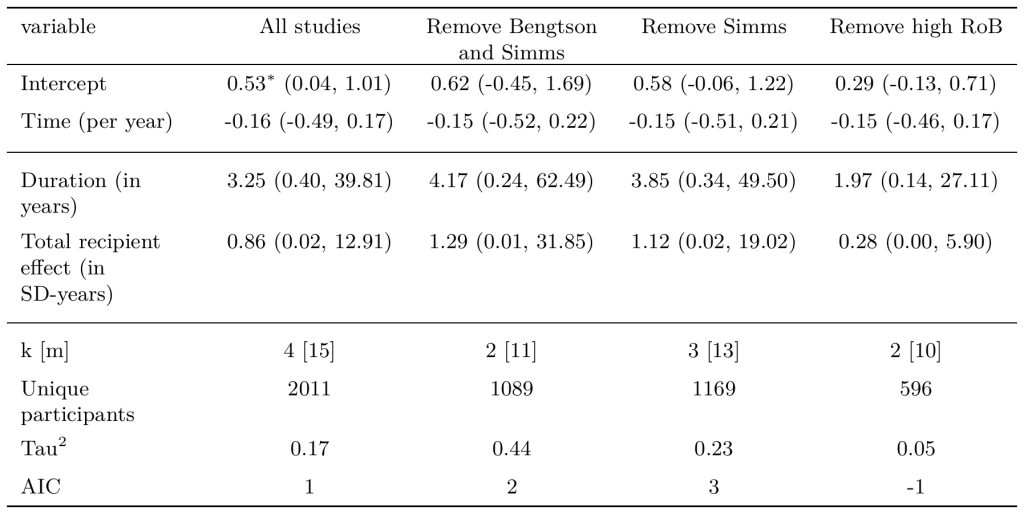
Note. All the effects presented above the first separation line are coefficients from the meta-analysis model. Their effects are in Hedge’s g (SD changes). The parentheses represent 95% confidence intervals. Statistical significance is represented such that * p < 0.05; ** p < 0.01; *** p < 0.001.
As aforementioned in Section 3.2.1, the inclusion of two RCTs which did not fully fit our criteria – Bengtson et al. (2023) or Simms et al. (2022) – is a conservative decision and so we keep them in order to have the most information possible.
Removing the two ‘high’ risk of bias studies (Chibanda et al., 2016; Simms et al., 2022) together reduced the effect. This is mainly driven by removing Chibanda et al. because Simms et al. does not change the modelling much alone. Nevertheless, as we explained in Section 3.2.1, we do not think this justifies removing these studies. Chibanda et al. is the most representative study of Friendship Bench, its risk of bias is likely a risk of downward adjustment, all the other domains would see Chibanda et al. rated as ‘some concern’ risk of bias, and we still find Friendship Bench to be cost-effective if we remove them. We do not think removing these studies is an appropriate decision.
4.2.2 StrongMinds causal evidence
We analysed Baird et al.’s (2024) effect sizes in a meta-regression modelWe use a meta-regression (see Section 2 and Appendix C) because there are multiple effect sizes across different outcomes measures and follow-up time. This allows us to have the results in SDs, estimate the trajectory over time for this source, and have comparable modelling to the other data sources. (see Table 7), the estimated effects are very small. The initial effect is positive and significantWhy is it significant when in Section 3.2.2 we mentioned that there was only one effect size that was significant? Because a meta-analysis can increase precision by combining multiple effects. Note that our multilevel structure would adjust for dependence between the effects. Although, there is only one study here so there is no heterogeneity, making a random effects model and a 3-level model the same., but the decay is non-significant. This leads to a total effect of 0.07 SD-years or 0.15 WELLBYs.
Table 7: Meta-analysis the Baird et al. data.
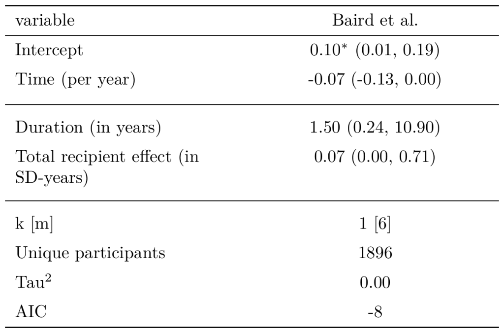
Note. All the effects presented above the first separation line are coefficients from the meta-analysis model. Their effects are in Hedge’s g (SD changes). The parentheses represent 95% confidence intervals. Statistical significance is represented such that * p < 0.05; ** p < 0.01; *** p < 0.001.
The controlled (but not randomised) study of StrongMinds’s own programme in Uganda (N = 371; Peterson et al., 2024) found a significant difference between the treatment and controls group of 6.21 points on the PHQ-9 scale at 6 months follow-up. This is much higher than the 0.30 points difference on the PHQ-8 found by Baird et al. at post treatment.
4.3 Charity-related pre-post
We use M&E pre-post data from the charities. This data is arguably the most relevant data available about the charities because these are the effects of the latest work from the charity. Hence, the M&E pre-post data could be more relevant than general RCTs in LMICs (because these are not about the charity directly) and RCTs of the charities (because these are not necessarily exactly how the intervention is currently implemented).
However, pre-post estimates (i.e., within-person effects) do not have a control group to compare the results to (i.e., do not have between-person effects), which means results will be inflated compared to RCT between-effects and, additionally, would lack causal explanatory power (Morris & DeShon, 2002; Cuijpers et al., 2016). Omitting a control group can confound the results; notably, participants’ levels of depression might reduce – to some extent – even without psychotherapy (i.e., spontaneous remission; Cuijpers et al., 2014), making the reduction in the treatment group (the within-effect) an overestimate if not compared to a control group (to calculate the between-effect). In order to make pre-post results (i.e., within-effects) more comparable with RCT results (i.e., between-effects) we need to adjust for this overestimation.
Ideally, we would use a synthetic control groups methodology. To do so, we would have to find individuals in the same context as the charities, who reported results on the same scales as the charities, who we can match on important characteristics to the clients of the charities (initial levels of mental distress, demographics, socio-economics, etc.), and who did not receive the intervention. We could not find data that would fit these demands. However, we do have data about control groups in our general RCTs of psychotherapy in LMICs.
So, we use a simpler, less ideal, ‘pseudo-synthetic’ control approach where we take RCTs from our general meta-analysis which use the same scales as the charities. We then take a weighted average of their control groups to form our pseudo-synthetic control group for the pre-post data. In other words, we use the averaged data from the control groups from other contexts (of varying similarity, at the very least in LMICs and using the same scales) to act as our control group for assessing the monitoring and evaluation data. This is not ideal, but it adjusts for issues of using pre-post data better than not using a control group. Thereby, this unlocks what could be the most relevant data. For more detail on the calculations, please see Appendix K.
We are very uncertain about our methodology here, and acknowledge that it is not a standard process. Nevertheless, we give little weight to the pre-post data (less than 17%; see Section 7) and we check how robust data sources are to different data sources (i.e, whether the estimated cost-effectiveness differs across each source of evidence; see Section 9.3).
4.3.1 Friendship Bench pre-post
For the M&E, we estimate an average initial effect of 0.12 (95% CI: 0.04, 0.19) SDs using our pseudo-synthetic control method. We use the duration from the general psychotherapy model – 3.48 yearsThis is from the model without the longterm follow-ups (see Section 4.1), – to estimate a total effect on the recipient overtime of 0.41 (95% CI: 0.14, 1.00) WELLBYs. This is potentially conservative considering the reference RCTs all were ‘enhanced usual care’ control groups rather than ‘nothing’ as is typically available to people in Zimbabwe.
4.3.2 StrongMinds pre-post
For the M&E, we estimate an average initial effect of 0.79 (95% CI: 0.74, 0.84) SDs using our pseudo-synthetic control method. This is larger than the initial effect in our general meta-analysis (see Section 4.1; and Section 5.1.4 for how our adjustments reduce this below the effect of the general meta-analysis). We use the duration from the general psychotherapy model – 3.48 yearsThis is from the model without the longterm follow-ups (see Section 4.1), – to estimate a total effect on the recipient overtime of 2.75 (95% CI: 1.71, 5.91) WELLBYs.
We think that the M&E effects here are at least somewhat informative because we think StrongMinds collects good quality M&E data, they were collected on a large sample of clients (almost all the clients, see Section 3.2.2) and StrongMinds’s M&E data has been validated by an external agency (see 2023 Q4 report). This external validation was a study of N = 792 clients in Uganda and Zambia where they found an average pre-post of -12.49 points (or, of -11.70 points if re-weighted according to the proportion of clients StrongMinds treats via peers and partners). Note that we used the most conservative of the pseudo-synthetic options available to us, so results may be even higher (see Appendix K2.2). Plus, as we explain in Section 5.1, we will add two rather severe adjustments for the potential that such results are replicated (0.51) and for response bias (0.85). Finally, note that we only give 16% of the weight to this pre-post result.
It is worth asking why the pre-post results are so different from the results from Baird et al. (2024). It is difficult to untangle, but the pre-post changes (-13.04 for StrongMinds; -5.27 for Baird et al.) suggest that the programme in Baird et al. was less effective (see Appendix K2.2 for more detail), reinforcing the idea that the programme in Baird et al. might simply be a failed implementation because of its contextWe acknowledge that an alternative could be that the M&E results are inflated, but we think that the issues with Baird et al. are more likely.. After treatment, the treatment group in Baird et al. had much higher levels of depression (7.90 points) than clients in StrongMinds’ M&E (2.49 points)StrongMinds’s M&E is on the PHQ-9 scale (a 27 points depression scale), so higher scores are worse. Baird et al. uses the PHQ-8, which is the PHQ-9 without the question about suicidal ideation, making it a 24 point scale (i.e., when linearly transformed, its results are higher). In the case of the post-treatment treatment group mean it would be 7.90 * 27/24 = 8.89..
5. Validity adjustments
Previously, we have explained the total effect as per the different sources of evidence. However, we cannot necessarily take these results at face value in our evaluation. In this section we discuss our validity adjustments, where we attempt to correct for methodological inadequacies and make our estimates more generalizable to the charity specific context. The results of the adjustments are summarised in Table 8. In the following sections we discuss the different adjustments and how they apply to the different sources of evidence.
Table 8: Summary of validity adjustments.
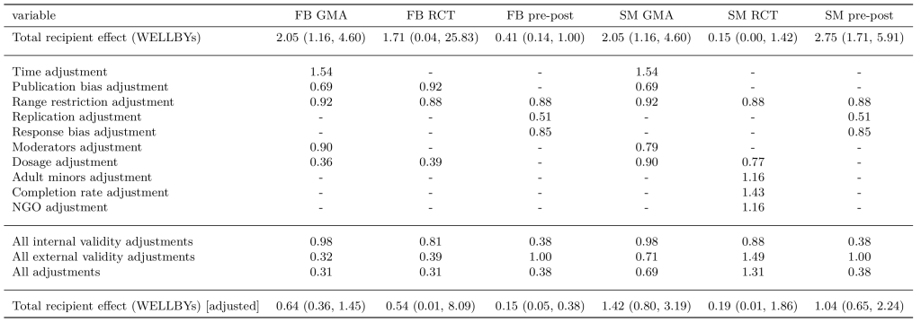
Note. Friendship Bench (FB) and StrongMinds (SM). The general meta-analysis (GMA; see Section 3.1) is used as an evidence source for both charities separately. This is when the results for the GMA starts diverging between the two charities because we apply different external validity adjustments. The parentheses represent 95% confidence intervals.
5.1 Internal validity
In this section we discuss internal validity adjustments, which are aimed at correcting for biases in the effects. These are separate from correcting for issues regarding a lack of relevance to the charity context, which we attempt to deal with in the external validity section.
5.1.1 Adjusting for extreme long-term follow-ups
As mentioned in Section 4.1 and Appendix D, we use the general meta-analysis model without the extreme follow-ups but adjust the total effect so that it represents a 50-50% weighting between the model with and without extreme follow-ups. We do so by applying an adjustment the effect estimated by the general evidence by 1.54. We only apply this to the general meta-analysis, we do not apply this to the charity-related RCTs and for the M&E pre-post. We are currently taking the decay rate implied by the charity-related RCTs at face value and for the M&E pre-post estimates we impute the duration from the general meta-analysis model without very long run follow-ups.
5.1.2 Adjusting for publication bias
Publication bias is “when the probability of a study getting published is affected by its results” (Harrer et al., 2021). Publication bias is widespread in social science generally (Franco et al., 2014). When it is identified, it should be corrected for. This is a complicated topic with many parts that we briefly summarise here, see Appendix E for more detail.
There are signs of publication bias in our meta-analysis of psychotherapy in LMICs - unsurprising given they are a general feature of academic work. Therefore we want to use a correction method to adjust the effect to better reflect the results if there was no publication bias. However, none of the methods perfectly fit the structure of our dataThe Nakagawa method (Nakagawa et al., 2021, correction) is the most appropriate for our modelling purposes because it can incorporate the multilevel modelling structure and the moderation over time. However, we do not think its greater compatibility with our modelling approach is sufficient grounds for us only using this method. It is still a new and relatively untested method. and no method of publication bias adjustment systematically out-performs the others (Carter et al., 2019; Hong & Reed, 2020)Performance is determined by measures of error or distance from the intended ‘true’ effect which is known in simulation studies because authors set the characteristics of the data that is simulated.; hence, it seems inappropriate to only pick one method. Instead, we use multiple methods and take an average of the adjustment that they suggest.
The methods suggest adjustments ranging between 0.38 and 0.99, except for the ‘p-curve’ method that suggests an increase (by a factor of 1.10)This is likely because the p-curve is particularly known to perform poorly under high heterogeneity (see Appendix E for more detail).. A range of results is to be expected from different models (Carter et al., 2019; Hong & Reed, 2020), as they operate in different ways. The naive average of these is 0.69 (a 31% discount)If we remove the two worst performing methods according to simulation studies, the Trim and Fill and p-curve methods, the adjustment remains very similar at 0.66 (a 34% discount)..
We do not apply the publication bias adjustment for Baird et al. (2024) because it is only published as a working paper and is pre-registered. We apply the publication bias adjustment to the Friendship Bench RCTsIdeally, we would have enough data to calculate the potential for publication bias within the charity RCT data itself. However, there are too few studies to make a meaningful analysis. There are many effect sizes, but these come from 4 RCTs, and only one publication bias method can account for MLM and moderators, that is the Nakagawa method (see Nakagawa et al., 2021). When we test the Nakagawa method on the Friendship Bench RCT data, it does not suggest that there is publication bias, and even suggests an upwards adjustment. but we proportionally reduce the discount by ¾ because ¾ of the Friendship Bench RCTs are pre-registered and seem to have, overall, followed their protocols. This reduces the adjustment to ¼*0.69 + ¾*1 = 0.92 (8% discount). We do not apply this to the pre-post data, but we do apply a replication adjustment instead (see Section 5.1.4).
5.1.3 Adjusting for range restriction
We use Cohen’s d and Hedges’s g, a common form of standardised mean difference, to standardise effect sizes in our meta-analyses. Variance plays a justifiable role in this method for standardisation; however, in practice, there is a concern with psychotherapy trials, which commonly only include participants who are mentally unwell. Namely, it selects participants based on a cut-off on the outcome of interest, the affective mental health (MHa) measure. This restricts the variance of mental health scores we observe compared to the alternative where a general population (both people who are well and unwell) is treated. This is not an issue with other interventions such as cash transfers, where recipients are selected based on another criteria, like poverty, which is not our outcome of interest (i.e., a direct measure of subjective wellbeing or affective mental health).
This artificial shrinkage in the variance of mental health scores very plausibly leads to an overestimate of psychotherapy’s standardised effect sizes. This phenomenon is referred to as ‘range restriction’ or ‘range enhancement’ (Hunter & Schmidt, 2004; Wiernik & Dahlke, 2020; Harrer et al., 2021) and can be corrected if one knows the variance in the target population. However, this is not the case for us because we have many different studies, with different measures, across different countries. Instead, we apply a general adjustment calculated from general trends in the restriction of variance for mentally distressed populations (see Appendix F). We used three panel datasets and two RCTs in LMICs (for 408,500 observations) to estimate the size of this bias. On average, the variance for individuals past the threshold for mental distress becomes 0.88 (12% smaller) of that of the general population’s variance. Because the variance is on the denominator, this inflates effect sizes by 1 / 0.88 = 1.14. Which means that we need to apply an adjustment factor of 0.88 (a 12% discount) to correct for this. We apply this adjustment to every source of evidence.
However, this discount will only apply to the effect sizes where participants were selected based on a mental health cut-off (either on the outcome scale or a clinician diagnostic) and where responses are given on affective mental health measuresNot subjective wellbeing because we did not find evidence of range restriction in our tests with subjective wellbeing measures (see Appendix F).. This is the case for all of the charity-related causal and pre-post data. However, this only represents 64% of effect sizes in our general meta-analysisThis represents 65% of the weight of the meta-analysis but we use the percentage of studies because it is close and easier to to understand.. Adding this correction suggests that, to adjust for psychotherapy inflating SMDs, the adjustment factor would be 1 * 0.88 * 0.64 + 1*(1-0.64) = 0.92 (a 8% discount).
See Appendix F for more detail about this adjustment.
5.1.4 Adjusting for replication
For the charity-related pre-post data, we apply a ‘replication’ adjustment of 0.51 (49% discount)Nosek et al. (2022) reports on multiple replication efforts in psychological sciences: Camerer et al. (2018, k = 21), Open Science Collaboration (2015, k = 94) and the Multi-Lab studies (1,2,3,4; k = 77). For each, there is an original effect size and a replication effect size, so we can calculate how large the replication effect is compared to the original effect (i.e., a proportion). We take a weighted average of these proportions, which suggest that replicated effects are 51% of the magnitude of the original effects. instead of a 0.69 (31% discount) publication bias adjustment. This is a somewhat subjective adjustment which corresponds to our general and sceptical prior that many results do not replicate. This is a broader issue than the publication bias adjustment. This is because we think there are relatively more incentives for an organisation to report favourable results of its programme than for the average researcher to embellish the effects of the intervention they are studying. There is also potentially more flexibility and less oversight in how an organisation collects and presents its data than for academia. This is not a specific stance on the charities themselves, rather, as charity evaluators, we start with a sceptical prior belief and apply the adjustment unless we have strong citable evidence that the risks are mitigated.
While we still apply this adjustment, we think there are some reasons to think that the charities are not misusing degrees of freedom:
- StrongMinds has had its pre-post data validated by an external agency (see 2023 Q4 report).
- StrongMinds’ M&E pre-post data represents almost all of their clients in the year (see Section 3.3.2 for more detail), making it unlikely that they selected results in a way that would substantially affect outcomes. The amount of data is very large, making it difficult to change the averages through simple data tweaks (i.e. p-hacking). Influencing the mean outcomes would require systematic manipulation to the data.
- Friendship Bench shared data from 2021 to 2024 with us, demonstrating transparency.
For readers who do not think this adjustment is appropriate, here are how the results would change:
- The adjusted total effect on the individual for Friendship Bench’s M&E pre-post data would increase (0.15 → 0.30 WELLBYs), which would still be the smallest of the three evidence sources, but a lot less small than it is now and closer to the two other sources of evidence (see Table 8 at the start of Section 5). Thereby, the overall effect for this source will increase (0.23 → 0.45 WELLBYs; see Section 6) and the cost-effectiveness for this source will increase (14 → 27 WBp1k; see Sections 7 and 8).
- The adjusted total effect on the individual for StrongMinds’s M&E pre-post data would increase (1.04 → 2.06 WELLBYs) and become the largest of the three sources of evidence (see Table 8 at the start of Section 5). Thereby, the overall effect for this source will increase (1.68 → 3.31 WELLBYs; see Section 6) and the cost-effectiveness for this source will increase (38 → 74 WBp1k; see Sections 7 and 8).
5.1.5 Adjusting for response bias
Respondents to surveys about their wellbeing could be prone to response bias (this usually concerns a type of response bias called ‘demand characteristics’). We estimate a response bias adjustment of 0.85 (a 15% discount; see Appendix I1 for more detail). However, we only apply this adjustment to the M&E pre-post estimates (see below). We do not apply this adjustment to our causal estimates (e.g., general evidence and charity-related evidence) for the following reasons. We are very uncertain about our estimate. Calculating an empirical adjustment for response bias is not as straightforward (see footnote for an explanation of the challenges)One major challenge is determining whether to make a fixed adjustment (e.g., 0.25 SD) or relative adjustment (e.g. 10%). The decision depends on whether you model demand effects as uniform, with participants inflating their scores by a constant amount, or proportional, in which the size of the bias depends on the size of the true effect. We are uncertain which model is more appropriate. Another challenge is determining whether the available evidence is generalizable to the current context. . We hope we can form a better empirical estimate in the future as we find more data on the topic. Furthermore, this would affect all the charities we evaluate (StrongMinds, Friendship Bench, GiveDirectly, etc.) in plausibly similar ways. We do not think there would be strong deviations in response bias between psychotherapy, cash transfers, and other interventions we analyse. So, it would not change the relative differences and we would have to apply it to every analysis. While we think this would be a useful addition to our methodology, we think we should wait to apply this adjustment broadly until we have better data on the topic.
We think estimates based on M&E data are more at risk for response bias than the RCT sources because the responders can plausibly connect the data collection process with the charity that has previously benefited them, and there may be organisational incentives to show positive outcomes. This seems like a reasonable precaution, especially in light of the high degree of speculation involved in our ‘pseudo-synthetic control’ methods for pre-post data (see Appendix K for more detail), and the fact that it represents a very small part of our final estimate.
5.2 External validity
External validity adjustments, which aim to make the estimates more representative of the anticipated effect of the charity programmes in practice, are applied to the general meta-analysis of psychotherapy in LMICs and charity-related causal evidence sources of data. In other words, we have a variety of studies in the meta-analysis, so we use that to predict what the effects would be for programmes with the characteristics of Friendship Bench or StrongMinds.
The charity-related pre-post data is not adjusted for external validity because it is representative of the charity programmes as they are practised (i.e., they have the right intervention and charity characteristics).
We summarise the differences in implementation between StrongMinds and Friendship Bench in Table 9. Then we explain how we adjust for these characteristics for each charity and each data source.
Table 9: Summary of differences in intervention delivered.
|
StrongMinds |
Friendship Bench |
|
|
Type of psychotherapy |
Interpersonal psychotherapy (IPT) Focuses on identifying issues in interpersonal relationships and resolving them, plus building skills to resolve them in the future. |
Problem Solving Therapy (PST) Focuses on identifying current problems and develops skills to understand the problems and learning the skills to logically solve them with concrete steps. |
|
Country of delivery |
Uganda and Zambia |
Zimbabwe |
|
Delivery method |
Group |
One-to-one |
|
Expertise of deliverers |
Lay therapist (either peers in the community or community health workers trained by clinicians to deliver the psychotherapy programme) |
Lay therapist (peer in the community, called ‘grandmothers’, trained by clinicians to deliver the psychotherapy programme) |
|
Average sessions completed (from the charities’ own M&E information) |
5.63 |
1.12 |
|
Access to good alternative to therapy |
No, we think this is unlikely. |
No, we think this is unlikely. |
|
Are the clients mentally distressed? |
Yes. Selected on depression scores (PHQ-9). |
Yes. Selected on general mental distress (depression and anxiety) scores (SSQ-14). |
Another difference between the charities is that StrongMinds delivers psychotherapy to 78% of its clients via partners; we adjust for this in the costs (see Section 8).
5.2.1 Adjusting for non-dosage charity intervention characteristics
We use our moderator analyses to adjust for the characteristics of the interventions (see Table 10 and Appendix G for more detail). We moderate for (A) group (vs individual) and (B) lay therapist (vs professional) delivery. While therapy in high-income countries is often delivered one-on-one, by specialists with years of training, resource constraints in LICs have led to the development of ‘task-shifting’, where lay therapists are used. Lay deliverers are trained by experts to deliver the manualised programmes of the charities (Vally & Abrahams, 2016; Galvin & Byansi, 2020; Chowdhary et al., 2020; Karyotaki et al., 2022; Purgato et al., 2023). Lay deliverers (and group format) helps reduce costs, increase the number of deliverers, and increase the number of patients treated. We selected the moderators based on theoryWe did not include modality (CBT, IPT, etc.) as a moderator because: (1) this model depends on us determining which modalities different studies belong to (many of which have hard to classify modalities), (2) most of the coefficients are imprecisely estimated, and (3) most of the evidence for PST, the modality for Friendship Bench, comes from the Friendship-Bench-related RCTs themselves, which would be too much like double counting. (rather than only statistical model comparison). The exception is moderating for Iran studies, which we think are biased, as we already explained in Section 4.1. We could have added other moderators, but they are less precisely estimated and the moderation would be less conservative (see Appendix G for more detail).
Table 10: Charity characteristic moderation.
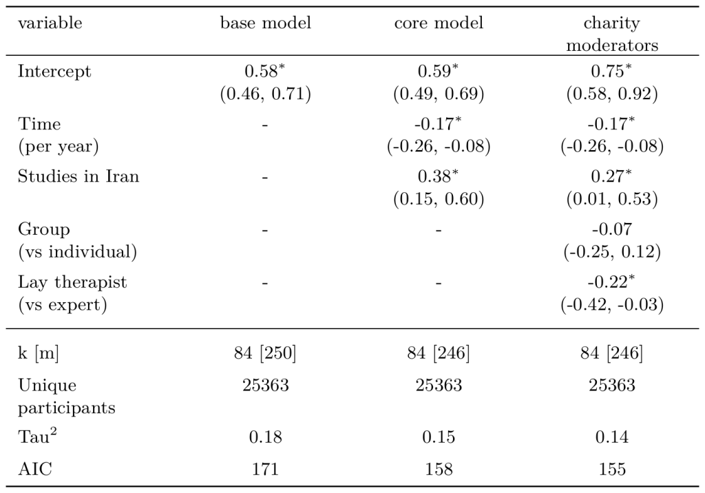
Note. All the effects presented above the first separation line are coefficients from the meta-analysis model. Their effects are in Hedge’s g (SD changes). The parentheses represent 95% confidence intervals. Statistical significance is represented such that * p < 0.05; ** p < 0.01; *** p < 0.001.
This shows that both group delivery and lay-therapist delivery reduces the effectiveness of the intervention. Note that these are features that also reduce the cost of the intervention (see Section 8) and allows for the charities to reach more people in need. Thereby, this is likely still an advantage for the cost-effectiveness of the charities. A moderately effective intervention will be more cost-effective (vs a very effective intervention) when the costs are low enough.
We calculate the adjustment by calculating the intercept adjusted for the different characteristics, which we then divide by the intercept in the core model.
Friendship Bench delivers 1-1 psychotherapy, via lay-therapist, to individuals with mental health problems, who have no enhanced alternatives to psychotherapy. We adjust the general meta-analysis of psychotherapy as source of evidence for Friendship Bench by 0.90 (10% discount) for using lay therapistsThe adjusted intercept is calculated as 0.75 (intercept) + -0.17 * 0 (setting time to 0) + 0.27 * 0 (not Iran) + -0.07 * 0 (not group therapy) + -0.22 * 1 (lay therapist) = 0.53. Therefore, the adjustment is 0.53 / 0.59 = 0.90..
StrongMinds delivers group psychotherapy, via lay-therapist, to individuals with mental health problems, who have no enhanced alternatives to psychotherapy. We adjust the general meta-analysis of psychotherapy as source of evidence for StrongMinds by 0.79 (21% discount) for using lay therapists and group formatThe adjusted intercept is calculated as 0.75 (intercept) + -0.17 * 0 (setting time to 0) + 0.27 * 0 (not Iran) + -0.07 * 1 (group therapy) + -0.22 * 1 (lay therapist) = 0.46. Therefore, the adjustment is 0.46 / 0.59 = 0.79..
We do not adjust the charity-related RCTs for these charity characteristics because the interventions studied in these RCTs have similar characteristics to how the charities implement their programmes (see Section 7 for more discussion about relevance)There are two deviations in the Friendship Bench relevant RCTs that we do not adjust for. First, all these RCTs provide some form of enhanced usual care (EUC) control. It often includes supportive information, sometimes even some aspects of counselling, and some HIV treatment support. As per our moderator modelling (see Appendix G), if we adjusted for this, we would apply a very small increase in the effect of these RCTs. We do not apply this for simplicity.Additionally, all of these RCTs target populations with HIV to some extent (Chibanda et al., 2016, did not specifically target individuals with HIV but 42% of the sample did have HIV).We find a non-significant reduction in effects when the population was individuals with HIV (see Appendix G for more detail).. We do adjust the charity-related RCTs for dosage (see Section 5.2.2) and the Baird et al. RCT for some extra adjustments (see Section 5.2.4).
5.2.2 Adjusting for dosage
The general evidence and the charity-related RCTs differ from how the charities implement their programme in terms of dosage. Dosage can be understood in two parts: intended number of sessions and actual attendance. For example, StrongMinds intended for participants to have 6 sessions, but participants attended on average 5.63 sessions, which is an attendance rate of 5.63/6 = 94%. In our general meta-analysis the average number of sessions intended is 7.18 and the attendance rate is 71%.
Ideally, we would build our dosage adjustment from two adjustments based on empirical evidence: one for intended sessions and one for attendance. We encounter limitations in modelling both of these:
- We can model the effect of intended sessions in our general meta-analysis (see Appendix G for a lot more detail). However, the estimate of the effect of dosage has greatly varied across different versions of this analysis. Notably, in this version, it is small, and not statistically significantFor the linear specification of the dosage, it is tiny and negative, but this changes to tiny and positive once one outlying high dosage (32 sessions) study is removed.. Cuijpers et al. (2013) also found a small, non-significant effect of the number of sessions in their analysis. So we cannot conclude much about dosage from this model and do not use it to calculate a dosage adjustment.
- We do not have sufficient data to model the effect of attendance. Only 17 studies reported attendance rates; we could not extract average attendance for the remaining 67 studies because authors do not report this information. For these 17 studies we find that the average attendance rate was 71% (range: 43% to 95%).
We considered many different possible calculations of the dosage adjustment (see Appendix G for more details). Because it is based on too few studies we do not use the average attendance as an independent adjustment but instead we merge the two adjustments into one by comparing the attended sessions in the charity to the intended sessions in the data source (e.g., 5.63 sessions attended for StrongMinds vs 7.18 sessions intended for the general meta-analysis).
Instead of relying on an uncertain coefficient from our moderator analysis we do a simple calculation of dosage, where we assume a logarithmic dose-response relationship. This would be ln(attended sessions in the charity + 1) / ln(intended sessions in the source + 1). We explain why we add +1 to the calculation in a footnoteAs a mathematical property, log(1) = 0, and log(0) is undefined. This means a dosage of 0 is unknown and a dosage of 1 will be calculated to have 0 effect. However, we know a dosage of 0 would have 0 effect, and we expect a dosage of 1 will have a positive effect, so we need to correct for this. Therefore, we adopt the approach of adding a constant, c = 1, to the log values, which addresses this mathematical complication by shifting the log scale up the number line. Doing so means that 0 dosage is calculated as log(0+1) = 0 and a dosage of 1 has a non-zero value. In this case, it means a dose of 1 will be 33% as large as a dose of 7, log(1+1)/log(7+1) = 0.33. It is possible that the true relative impact of the first session is bigger or smaller than this, but we think this provides a very reasonable estimate, given that we expect that the first session of psychotherapy will provide the most benefit..
This is a moderate adjustment (but more conservative than if we used our modelling of attendance and intended sessions). In our sensitivity analyses (see Section 9.3) we also consider no adjustment for dosage (as we cannot calculate a stable one from our model) which is more favourable, and one more conservative based on a simple linear calculation devoid of empirical information: attended sessions / intended sessions, which is more conservative.
Friendship Bench clients complete, on average, 1.12 out of 6 maximum sessions of psychotherapyThis is information provided to us by Friendship Bench based on their general M&E data.. This is a major source of our uncertainty about how effective the Friendship Bench programme might be, so we elaborate on it in Section 5.2.3. While this might mean that some clients stop attending because they do not find the sessions helpful, we think there are plausible reasons to believe that few sessions can be helpful. Notably, PST (which is what Friendship Bench delivers) is built on identifying and solving problems from the very first session. Hence, providing 6 sessions is not necessarily the aim, but solving problems that affect clients’ mental health is. We consider 6 sessions to be the intended sessions as a conservative measure.
This attendance of 1.12 sessions is substantially less than the average 7.18 intended sessions in the general meta-analysis data, so we adjust for the general meta-analysis for Friendship Bench by an adjustment of ln(1.12+1) / ln(7.18+1) = 0.36 (i.e., a 64% discount). This attendance is also less than 6 intended sessions in each of the Friendship Bench related RCTs, so we also adjust the Friendship Bench relevant RCTs by ln(1.12+1) / ln(6+1) = 0.39 (61% discount). This seems like very low attendance (and thereby, we assume, very low dosage).
StrongMinds clients attend, on average, 5.63 out of 6 intended sessions of psychotherapyThis is information provided to us by StrongMinds based on their general M&E data.. This is less than the average 7.18 intended sessions in the general meta-analysis of psychotherapy data, so we apply an adjustment of ln(5.63+1) / ln(7.18+1) = 0.90 (i.e., a 10% discount).
We apply this adjustment a bit differently for the Baird et al RCT, because here we have the actual attendance data, so we do not have to rely on intended sessions as a rough proxy. Participants who attended at least one session attended, on average, 10.56 (10.56/14 = 75%) sessions in Baird et al. (2024; calculated from their Table A2), which is higher than the actual average of 5.63 (5.63/6 = 94%) sessions from StrongMinds recipients, but actually a much lower attendance rate. Because we have attendance rate information for the Baird et al. RCT, we use a more sophisticated and accurate dosage adjustment here. Instead of comparing 5.63 to 14 (i.e., the intended number of sessions in Baird), we compare 5.63 to 10.56 (i.e, the average attended number of sessions in Baird), which results in an adjustment of 0.77 (33% discount)Note that this 10.56sessions is the average number of sessions participants who attend at least one session. If we widen this to the number of sessions for all participants (including non-compliers who attend 0 sessions), this is much lower with5.94 (5.94/14 = 42%) sessions on average. This would suggest an adjustment of 0.98 (2% discount). If we compared it to the intended number of sessions 14 – thereby ignoring the information about actual attendance – the adjustment would be 0.69 (31% discount).. This is more detailed but less conservative than what we apply for the other sources of data. Nevertheless, we think it is appropriate to use the actual attendance for Baird et al. because doing so is more relevant and because there are big issues with non-compliance that we think are unrepresentative of how StrongMinds operates (see Section 5.2.4).
Note that we are not particularly concerned with dosage for StrongMinds because it has a high attendance rate. Furthermore, StrongMinds has communicated to us that their decision to deliver 6 sessions comes after doing A/B testing which showed that they could reduce the number of IPT sessions without reducing much of the effect by grouping participants according to specific triggers for their mental distress. The A/B testing has not yet been published so we do not yet know the results.
5.2.3 Discussing Friendship Bench’s low dosage
The very low attendance (and therefore, we assume, low dosage) from Friendship Bench, where recipients attend on average 1.12 sessions instead of the maximum 6 sessions is our largest source of uncertainty concerning our estimate of the effectiveness of Friendship Bench. While this could be a sign that some participants have barriers to attendance or might not find sessions helpful, we discuss here why we think it is plausible that this low dosage can still represent effective treatment. Note that we remain very uncertain about this and would revise these numbers if new data or considerations came to light.
In the points below, we summarise the reasons why we think it is still plausible that Friendship Bench is cost-effective at improving global wellbeing:
- The harshest possible dosage adjustment is 1.12/7.18 = 0.16 (a 84% discount) – which we consider in our robustness checks (see Section 9.3) – still has Friendship Bench as cost-effective with 23 WBp1k (i.e., about 3x cash transfers). Hence, our overall conclusion that Friendship Bench is cost-effective is robust to the type of calculation selected.
- There is research by Schleider and colleagues (Schleider & Weisz, 2017; Schleider et al., 2022; Fitzpatrick et al., 2023) to show that even single session therapy can be effective, even in LICs (Osborn et al., 2020; Venturo-Conerly et al., 2022). Our adjusted effects for Friendship Bench are close in magnitude to the effects found in this literature. Although note that these are interventions designed to be just one session.
- We think that it is plausible that low attendance can still be impactful because the first few sessions can play an important psychoeducative role (i.e., about one’s understanding of mental health and how to improve one’s mental health), especially in LICs where psychoeducation is potentially lower. This was witnessed in our site visits (see Section 9.4) where clients mentioned how helpful the intervention was. Furthermore, StrongMinds staff mentions that clients often say – prior to attending psychotherapy – that their mental health problems came from curses.
- The first session of problem solving therapy (the programme Friendship Bench uses) does involve an entire process of discussing a problem and making a plan to address it, it is not just an introduction. It seems likely that people address their most important issues in the first session, while subsequent sessions would deal with less important issues.
- Thereby, providing 6 sessions is not necessarily the aim, but solving problems that affect clients’ mental health is. We consider 6 sessions to be the intended sessions as a conservative measure. The max number of sessions in the pre-post data Friendship Bench shared with us was 4 sessions, not 6. For some clients this might be because they have barriers to continuing, but for others it might be because they have solved their problems by then.
- The Friendship Bench 2023 pre-post data source is a result directly for this low dosage (with all the caveats of using this data source; see Appendices K and O1). While the lowest of the three data sources, is still more cost-effective than cash transfers with 13 WBp1k.
- Friendship Bench have told us that they believe low attendance is not necessarily a problem because some clients only do a few sessions because they feel like it has helped them and they do not find more sessions necessary. Other clients, however, encounter barriers like transport, which suggests the attendance could be improved for some clients. Friendship Bench have told us that they plan on improving uptake. We are keen to see improvements in these areas in future data reports.
|
Crucial consideration: Friendship Bench’s low attendance, and how to adjust for it, is a major source of uncertainty in our analysis. We elaborate on the points raised above in Appendix H. |
5.2.4 Additional adjustments for the Baird et al. RCT
We adjust the results from Baird et al. for three additional factors.
First, we adjust results because there are important issues with compliance in Baird et al. (2024; see their Table A2), separate from the absolute attendance discussed previously. Only 56% of participants in the treatment group attended any sessions (i.e., 44% attended zero sessions). This low compliance is likely unrepresentative of the high attendance in actual StrongMinds groups (5.63 out of 6 sessions, with only 4% of clients attending zero sessions)Baird et al. (2024)argued that this 44% non-compliance rate is not as bad as Bandiera et al. (2020), where 79% attended zero sessions. However, Bandiera et al. deployed an “Empowerment and Livelihood for Adolescents” (ELA) programme, not group psychotherapy for depression + ELA programmes like BRAC did in this study by Baird et al. Moreover, the low attendance in Baird et al. (2024) is also much lower than in Bolton et al. (2003) – an RCT of a programme very similar to that which StrongMinds delivers because it delivers task-shifted group IPT to adults in Uganda – as recognised by Baird et al. (2024, pp. 13-14): “The share of participants that attended a high share of sessions is lower, however, than that reported in Bolton et al. (2003) among adults in rural Uganda. In that study, 54% of the participants attended at least 14 (or 87.5%) of the 16 total sessions, compared with only 28% of the participants in our study, who attended at least 12 (or 85.7%) of the 14 total sessions.”.
Baird et al. (2024; see their Table A4) present results of a LATE analysis (i.e., treatment on the treated, an analysis on compliers), which provides the results on those who actually attended one or more sessions. This is different from the main results we use: the results on all the Baird et al. participants, including participants who attended zero sessions (i.e., ‘intention to treat’). Note that we typically prefer intention to treat estimates – which are the analyses from which we extract results for every other study in our analysis when possible – because they are more likely to represent the real world problems with implementations (e.g., non-compliance suggests a flaw in the programme). However, in this case, we think that the very low compliance in Baird et al. (2024) is less, not more, representative (i.e., externally valid) of implementation by StrongMinds because of M&E data from StrongMinds suggesting high participation; hence, we want to adjust for this. We return to how (un)representative this low compliance is in Section 7.3.
We extracted effect sizes from the LATE analysis and meta-analytically modelled these as we did for the results on all the Baird et al. participants (i.e., including participants who attended zero sessions) in Section 3.3.1. This resulted in a total effect on the individual of 0.21 WELLBYs, which – while still very small – is larger than the 0.15 WELLBYs for all participants. We think that the treatment on the treated results will be more representative of StrongMinds than the results on all participants (including participants who attended zero sessions). Therefore, we apply an adjustment of 0.21/0.15 = 1.43.
|
Crucial consideration: Note that while we adjust for this, this does not mean that it solves this issue. We still think it is very problematic that the Baird et al. trial has high non-compliance which is unrepresentative of how StrongMinds operates (see Sections 3.2.2 and 7 for more detail). |
Second, the population of the Baird et al. (2024) RCT was adolescent girls, whereas StrongMinds primarily treats adults. Psychotherapy typically has larger effects on adults than adolescents (e.g., Cuijpers et al., 2020). We adjust for this by using the Metapsy database to run an analysis comparing results on adults and adolescentsThis analysis is mainly in HICs, there is no one dataset that combines results for both adolescents and adults in LMICs that we could use.. We find that, on averageAfter removing outliers with g> 2 SDs., the effect for adults (0.61; 95% CI: 0.57, 0.65; k = 422) is higher than for adolescents (0.51; 95% CI: 0.38, 0.64; k = 45) by a factor of 1.20. Based on data provided to us by StrongMinds, we calculate that 18% of patients treated are adolescents, thereby we adjust this factor down to 1*0.18 + (1-0.18)*1.20 = 1.16. Hence, we adjust the results upwards by this factor.
Third, StrongMinds had an external validation of their M&E data for the year (see 2023 Q4 quarterly report; N = 792). In it they find that the pre-post scores are smaller for NGO partners than the average of the rest of the delivery contexts. We think BRAC is an NGO partner, thereby, to make the results more representative of StrongMinds’s general effects, we adjust by the ratio of the pre-post effects StrongMinds report between their NGO and non-NGO clients: 1.16We use the information provided in the 2023 Q4 quarterly report which is pre-post split across partner types from the external validation study. The pre-post scores for NGO partners (-9.70 points on the PHQ-9) are smaller than the average of the rest of the delivery contexts (-11.70 points on the PHQ-9, on average, weighted by the proportion of clients treated by the different delivery methods: NGO partners, Government partners, peer facilitators, StrongMinds staff). This suggests an adjustment of 1.21. Nevertheless, StrongMinds does treat 24% of their clients via partners, so we adjust the adjustment to be (1*24%)+(1.21*76%) = 1.16. Note that this is not the same pre-post data we use as our third source of evidence, where instead we use pre-post collected on almost all of the StrongMinds clients (see Section 3.3.2). Thereby, we only use this information to calculate the adjustment..
|
Crucial consideration: After all these adjustments, the total effect on the individual for Baird et al. (2024) increases from 0.15 to 0.19 WELLBYs. Typically, our adjustments tend to reduce the effects, but in this case we think that adjusting upwards is what makes the Baird et al. results more externally valid (see Section 7 for more discussion about Baird et al.’s relevance, as well as Appendix O1 for how the cost-effectiveness would change without these adjustments). |
5.3 Validity adjustments we do not apply
There are a few validity adjustments that we do not apply here. We briefly mention them and why we do not apply them.
No adjustment for differences between mental health and subjective wellbeing measures
Most of the data in this analysis comes from affective mental health (MHa) measures rather than classical subjective wellbeing (SWB) measures. Ultimately we are interested in wellbeing, but the dearth of data on classical SWB measures means we need to broaden the scope of our included data. Theoretically, MHa measures ask people to report about negative affect (e.g., low mood) which seems highly relevant given our interest in happiness. Moreover, we have investigated this issue empirically. In a report (Dupret et al., 2024), we have shown that results on MHa outcomes do not overestimate results on SWB outcomes (if anything they slightly underestimate), which reassures us that using MHa and SWB as 1:1 equivalents in our results is an acceptable compromise considering the data landscape. We used data from this meta-analysis, our meta-analysis on cash transfers, a meta-analysis of psychotherapy in HICs (Boumparis et al., 2016), and multiple meta-analyses of psychological interventions in HICs.
No adjustment for differences in scale between RCTs and charity contexts
The charities operate at scales much larger than those of RCTs. It is plausible that at that scale, the effect would be lower in the charities than in the RCTs. However, we find very little empirical evidence that would satisfy us in determining an adjustment here. Furthermore, it is likely that the charities iterate, refine and maintain the quality of their intervention as their scale. The pre-post data from the charities suggest that they do still have large impacts even at their current scales (see Section 4.3). For these reasons, we do not apply an adjustment here (see Appendix I2 for more detail).
No adjustment for charity recipients otherwise being successfully treated
We care about the counterfactual impact of the interventions we evaluate (i.e., what would have happened if the charity or intervention did not take place). Would recipients of StrongMinds and Friendship Bench have received just as effective treatment anyway? If yes, then the charities have no counterfactual impact. However, we do not think this is much of a concern for several reasons. The standard of care is very low in LMICs. Moitra et al. (2022) estimates that 8% of depression cases are treated in LMICs, and only 3% are adequately treated. Given that most of our control groups are control groups where participants receive no extra support, we think that our model already accounts for the benefit of the alternative treatment. Our final consideration is that for every patient StrongMinds or Friendship Bench “take” from the reportedly overcapacity government clinics or the alternative provider of mental health treatment, those providers have the capacity to treat more patients, which would be a counterfactual bonus. Overall, we do not apply a counterfactual adjustment.
6. Household spillovers
The direct recipient of an intervention may not be the only person impacted. Indeed, if the direct recipient benefits, it seems plausible that in many cases those living with the recipient will also benefit (i.e., household spillovers). In which case, the overall effect of the intervention is likely underestimated by only focusing on the recipient effects. Moreover, spillovers can be greater or lesser for one intervention: our previous working has found that cash transfers have a relatively bigger spillover effect than psychotherapy (McGuire et al., 2022b), so we can’t just assume that every intervention has the same spillovers. Hence, we estimate spillovers to better capture the total effect of charities and interventions. However, spillovers are a highly neglected area of research and the data available does not allow for as good an estimation as for the individual effects.
In this section we briefly present our estimates of the spillover effects of psychotherapy. This is a summary of our analysis, which is documented in Appendix M.
6.1 Data
We searched for studies that reported results on household members as part of our systematic review and as part of our previous analysis of spillovers (McGuire et al., 2022b). We found a total of k = 6 interventions (m = 38 effect sizes, N = 16,445 unique participants, O = 35,497 observations). Most (83%) of the observations come from one study, Barker et al. (2022, O = 29,320).
6.2 Estimating the household spillover effect
Broadly, we combine two estimates of the household spillover effect based on two types of analyses:
- An analysis that takes the naive meta-analytic average of the highest quality studies.
- An analysis that separately estimates the spillover for each type of household role.
6.2.1 Naive meta-analytic average
Our estimate for the household spillover ratio is 11.79% if we only take the estimates from the meta-analytic average of the highest quality studies, Barker et al. (2022; spouse to spouse spillovers) and Bryant et al. (2022b, n = 714; adult to child spillovers). We prefer focusing on these studies because all other studies have characteristics that make a naive aggregation questionableThe three previously included studies have small sample sizes (Kemp et al. 2009, n = 24; Swartz et al. 2008, n = 47) and a low quality design. Mutamba et al. (2018) has a larger sample size (n = 116 to 142 for children and caregivers), but it also is notably not a randomised controlled trial, just a controlled trial. Of the new studies the results of the Betancourt et al. and McBain et al. combination find larger effects on the household member (0.00, 0.86 SDs) than the direct recipient (0.02, 0.02 SDs). This seems anomalous. While Bryant et al. (2022b, n = 714) takes place in a refugee camp, we confirmed an extraction point with authors that lead to a plausible spillover effect and so we combined it with Barker et al. (2022).. However, averaging these studies together neglects how different spillover pathways might present different patterns of results.
6.2.2 Pathways analysis
We also conduct an analysis where we attempt to separately estimate the spillover effect for each type of household relationship (i.e., different pathways) such as spouse to spouse, parent to child, and child to parent. See Appendix M for more detail. This includes the aforementioned RCTs, and we also reference a broader, non-RCT evidence base composed of five observational studies and two natural experimentsThe observational evidence comes from five studies of panel datasets with a total sample size of 31,632 (Powdthavee & Vignoles, 2008; Webb et al., 2017; Chi et al., 2019; Mcnamee et al., 2021; Eyal & Burns, 2018)and two natural experiments with a total sample size of 7,937 (Clark et al., 2021; Hinke et al., 2022). See Appendix M for more detail. (which we could not directly add in our naive average). Combining the different pathways of spillovers within a household depends on assumptions about the household composition (e.g., how many adults and children are in the household?). We use United Nations Population Division (UNPD, 2022) data about household size and composition to weight the different pathways. We estimate that if an adult receives psychotherapy, the average household spillover ratio will be 20.69%.
6.2.3 Synthesis and results
We (the authors of this report) are evenly divided on how to interpret the spillover results. Half the team endorsed a 12% estimate based on the average of the two best studies and the other half supported the 21% estimate based on the pathways analysis. Due to time constraints, we settled on assigning equal weights to both approaches and will revisit this analysis in the future. This results in an estimated household spillover ratio for psychotherapy in LMICs of 16%.
We think our estimate largely relies on relatively weak evidence compared to our estimate of the direct effect on the recipient (see Section 9.2). Notably, we assess the overall quality of evidence of the spillover evidence to be ‘very low’ (see Appendix J6 for more detail). This is primarily due to there being so few studies, especially RCTs, available on this topic. Therefore, we do not conclude that this estimate is the ‘true’ spillover ratio for psychotherapy, nor that this is an upper or lower bound, but only that this is a very uncertain estimateIn order to make the uncertainty estimates of our analysis of the psychotherapy charities comparable to that of GiveDirectly (see our website for more comparisons between charities), we need to induce some uncertainty around the spillover ratio estimate. However, our current analysis does not lend itself to an easy estimate of uncertainty. As a placeholder, we estimate the uncertainty of the spillover ratio in our Monte Carlo simulations with a beta distribution with a 95% CI of 0% to 50%, representing that we are very uncertain but that we think that the results could not be above 100% or below 0%. that could easily be updated with new evidence.
We hope to update this estimate if higher quality evidence about household spillovers is collected and becomes available – we know of one upcoming spillovers study and hope for more because this research area seems highly neglected. Spillovers can represent a large part of the effect, and so it is disappointing that there is so little evidence for this important part of the analysis. See our website for more detail about, and comparison with, the spillover ratios of other charities.
6.3 Overall effects: Adding spillovers
We apply the spillovers ratio to every source of data with the following equation:
Household effect = Total effect on recipient * spillover ratio * non-recipient household size
Non-recipient household members are the people in the household other than the recipient of psychotherapy. We calculate this by estimating the household size for the principal countries in which the charities operate and subtract 1 for the recipient member. We use UNPD (2022) data about household size and use a linear regression to predict the household size in 2024.
Then we can calculate the overall effect on the household with the following equation:
Overall effect = total effect on recipient + household effect
Note we do not attempt, here or in general, to calculate wider societal effects beyond the household. We lack data for this and it would be extremely speculative. It seems plausible that, in most cases, the lion’s share of the benefit of an intervention will be felt by the direct recipients and their household.
6.2.1 Friendship Bench
Friendship Bench primarily operates in Zimbabwe. See Figure 9 for our estimation of the household size and Table 11 for the results of the spillover analysis for Friendship Bench.
Figure 9: Analysis of household size in Zimbabwe for Friendship Bench recipients.
Note. The solid lines are the linear model. The dotted lines represent the predicted value in 2024.
Table 11: Overall effect for Friendship Bench data sources.
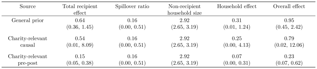
Note. Spillover ratio is a fraction, non-recipient household size is a number of individuals, the other values are in WELLBYs. All these results are after validity adjustments. The parentheses are 95% confidence intervals.
6.2.2 StrongMinds
For StrongMinds’s household size, we use the average household size for the African countries in which StrongMinds directly operates (Uganda and Zambia), weighted by their relative share of operations in these countries (70% Uganda and 30% Zambia). For this calculation we ignore the 3% of StrongMinds operation (through partners) in Nigeria, Kenya, and Ethiopia. We combine data from the UNPD and the Uganda National Survey Report of 2019/2020 (Figure 2.5 of that report; which is not included in the UNPD data).
See Figure 10 for our estimation of the household size and Table 12 for the results of the spillover analysis for Friendship Bench.
Figure 10: Analysis of household size for StrongMinds recipients.
Note. The solid lines are the linear model. The dotted lines represent the predicted value in 2024. The teal dots represent data from the UNDP. The red points represent data from the Uganda Social Survey.
Table 12: Overall effect for StrongMinds data sources.
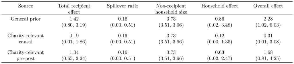
Note. Spillover ratio is a fraction, non-recipient household size is a number of individuals, the other values are in WELLBYs. All these results are after validity adjustments. The parentheses are 95% confidence intervals.
7. Weighting results from different data sources
7.1 General methodology
We are trying to estimate the true effect of the charities, using three different sources of evidence. However, aggregating estimates from different evidence sources (i.e., assigning weights) is an unsolved methodological problem with no standard best practice. The challenge is that each data source differs not only in statistical uncertainty (i.e., how precisely they estimate the effect), but also on hard-to-quantify qualities (e.g., how relevant the data source is to the charity). For example, the general evidence includes many RCTs, and the effect is measured relatively precisely; but, the studies have less relevance to how the charities operate. On the other hand, the charity M&E data is extremely relevant, but the data is lower quality because it does not come from an RCT.
Our approach to assigning weights involves a combination of empirical weights to account for the statistical uncertainty and subjective judgments to account for hard-to-quantify qualities such as relevance. In brief:
- We calculate empirical weights for the different sources according to their statistical uncertainty (i.e., the more certain, the more informative a source, the more weight it will have). We do this by using Bayesian updating, and form ‘Bayesian-informed weights’. We use this as our starting point.
- However, the empirical weights do not account for other sources of uncertainty that are hard to quantify into weights. For example, the relevance of the data source. So next, we subjectively adjust the Bayesian-informed weights based on hard-to-quantify qualities of the evidence sources which are not captured by statistical uncertainty.
- Four different researchers (Joel, Samuel, Ryan, and Michael) provided subjectively-adjusted weights and then we averaged their weights together. To form their weights, the researchers consulted the same shared information about each data source. The researchers assigned their weights independently, and then discussed and updated their weights together.
We expand on these steps below.
Empirical weights using Bayesian updating
Our method starts with calculating empirical weights for the different sources according to their statistical uncertainty. Statistical uncertainty is the spread around statistical estimates, represented by measures such as standard deviations, standard errors, confidence intervals (or credibility intervals, in Bayesian parlance). This captures an important feature: more precise (certain) estimates should influence our beliefs more.
We quantify the statistical uncertainty into Bayesian-informed weights using Bayesian updatingThere are alternative methods we could have used for weighting statistical uncertainty. For example, we could have simply used sample size, but this misses out on the combining of uncertainty from the initial effect and the trajectory over time. We get the impression that in academia, the preference might have been for combining all RCTs into one big meta-analysis instead of treating each source as separate. We think there is some value in treating each source as separate. Note that if we did simple weights based on sample size or put everything in one big meta-analysis, this would give weights of 12% or less to the charity-related RCTs (i.e., less than what we give with our method). Hence, by treating the sources separately we are already giving a lot of weight and importance to the charity-related sources of evidence relative to the general meta-analysis. See Appendix L for more detail. . In a Bayesian approach, you have a prior belief about the world that is more or less certain, and when you are exposed to new data (which is also more or less certain), you ‘update’ (change) your belief according to the relative certainty of your prior and the data to form a new posterior belief.
In this case, we consider the distribution of the effect for the general meta-analysis as the prior and the distribution of the effect for the charity-related RCTs as the likelihood (or new data) and combines them using statistical uncertainty, according to Bayes’ Rule, to form a posterior distributionWe did not use prediction intervals as some critics suggest because, until strong evidence to the contrary is presented, this approach is not conceptually appropriate, not practically appropriate, and would not change results much. See Appendix L1.2 for more detail.. We use a typical algorithm, Grid Approximation. Through this process we can quantify the weight by which the two evidence sources influenced the posterior. See Appendix L for more detail.
Note that there is no initial Bayesian-informed weight for the M&E pre-post data (see footnote for more detailWhile we could determine quantitative weights between the three sources of evidence, there are issues that make any purely quantitative weighting with the M&E pre-post data unreasonable. There are important limitations in our methodology for the M&E pre-post data (i.e., it is non-causal and we are uncertain about our pseudo-synthetic control methodology) and to calculate the total effect on the individual we are imputing the duration from the general evidence for psychotherapy, which means the statistical uncertainty for the M&E pre-post is not fully independent from the general evidence (see Appendix K). Therefore, we do not think that the statistical uncertainty estimated for the M&E data is appropriate for this exercise. Instead, after we calculate a Bayesian-informed weight between the two causal sources of evidence, raters allocate some weight to the M&E pre-post subjectively.), so weight assigned to the pre-post is purely done through our subjective adjustments to the weights – usually set by moving some of the weight from the general evidence. While the M&E pre-post data is the most relevant source of data, we do not give it too much weight because it is non-causal (and we are unsure about our pseudo-synthetic control methodology to deal with this).
Subjective adjustments to the weights
These Bayesian-informed weights serve as our statistical and quantitative starting point in determining our weights. However, there is one major drawback: these Bayesian-informed weights only capture statistical uncertainty (measurement error and inherent randomness), but do not capture uncertainty that has no clear way of being translated into statistical uncertainty (which model is more accurate, which theory is true, which data are more relevant to the question at hand, etc.).
To account for these hard to quantify characteristics, we considered each evidence source according to the GRADE criteria (Schünemann et al., 2013)This is a list of criteria used for evaluating the quality of evidence. We use it to evaluate the quality of evidence in Section 9. Here, we use it to give us a structure of which characteristics to consider in our weighting.: study design, risk of bias, imprecision (i.e., statistical uncertainty – already captured by the Bayesian-informed weights), inconsistency (i.e., heterogeneity), indirectness (i.e., relevance), and publication bias (see Appendix L1.3 for more detail). These criteria address major sources of uncertainty about evidence that we want to integrate in our weighting processUnfortunately, we could not find clear, precedented methods for converting these broadly qualitative factors (like ‘relevance’) into quantitative weights. Typically, GRADE criteria are used as qualitative assessments. Until further methods are developed, we believe our best bet is to rely on our best judgement and use information from these factors to subjectively adjust the Bayesian-informed weights for each evidence source
One alternative would have been to create a rubric for each qualitative criteria we might consider. Then each researcher would give a quantitative score for the different evidence sources across these criteria. For example, we could have rated ‘relevance’, ‘quality’, etc. with scores of (for example) 0 to 2. It has an advantage in that readers could more fine-tunely consult the elements that go into our weighting. We did consider this initially, but abandoned the idea for the following reasons. First, it is very time consuming, which is a problem considering the limited gains. Second, the quantification this method proposes seems more like a veneer because it engenders many technical questions. It is unclear how to grade the different steps of qualitative aspects. Should quality be classified as 0, 1, 2 or 0, 2, 3 (making it less important), or 0, 1, 4 (making it more important)? Should an RCT be worth X or Y times more than a pre-post? These are unanswered and somewhat subjective questions. Doi and Thalib (2008) propose something similar to this but where these scores are then used to adjust the weights directly in the meta-analysis (rather than to combine separate overall effects like we do in our analysis)..
We gave each researcher some freedom in how exactly they constructed their subjective weights, as long as they consulted all the relevant information from the GRADE ratings and provided weights that sum to oneSome of us directly set general weightings (i.e., subjectively adjusted the Bayesian-informed weights in their minds and then gave X% in total to the general evidence, and so on). Others built their weights with direct mathematical subjective adjustments (for each of the different relevant GRADE criteria) to the Bayesian-informed weights (e.g., -X% to the general evidence for lack of relevance). Some of us also used equivalent bets or other such techniques to internally test their subjective weights. We used the average of informed subjective weights provided from the four researchers (Joel, Samuel, Ryan, and Michael). . The researchers independently provided weights and then discussed their weights in a manner inspired by the Delphi methodThe Delphi methodis a forecasting technique that involves multiple rounds of asking a group of respondents for their views. Feedback is aggregated and shared with the group after each round to refine and converge on a consensus. We also did rounds of reporting views, discussing views, and updating views. However, we did not have a formal structure., and updated the weights based on discussion.
How our subjective adjustments differed from the Bayesian-informed weights
The Bayesian-informed weights give a lot of weight to the general evidence about psychotherapy in LMICs (see Sections 3.1 and 4.1). We think this is plausible, and sensible Bayesian epistemics to not ignore general knowledge about an intervention. Just like general information about anti-malaria bednets could inform us about a charity deploying bednets, general information about psychotherapy can inform us about these charities. Furthermore, the general evidence is more statistically certain than the other sources of data, it represents much more information than the other data sources. However, the charity-related causal evidence and the charity-related pre-post evidence are more relevant than the general evidence; hence, we adjust the Bayesian-informed weights in their direction by taking weight from general evidence and giving it to the other two sources. Therefore, these two sources of evidence benefit the most from the introduction of hard-to-quantify qualities such as relevance.
We recognise that our weighting method is an imperfect solution to an unsolved problemWe had our methodology reviewed by statisticians from Statistics Without Borders, a volunteer organisation that provides statistical consulting. They agreed that this is not a solved issue and that we are taking a reasonable approach given the constraints we have. They have given us blueprints to develop an even more sophisticated (but time consuming) process which uses more quantification and more Bayesian processes.. We hope that, by using the formal statistical uncertainty weights, the structure of GRADE, and the average of multiple weights, we have provided a reasonable set of subjective weights.
|
Crucial consideration: Because we are uncertain about this part of the methodology we also provide information about how sensitive the results are to the weightings (see Section 7.4). We are aware that others might provide different weights. Some might want to put more weight on the charity-related RCTs and/or pre-post data. We invite them to consider our reasoning about the relevance in the subsections below. We strongly suggest that readers who intuitively disagree with our weightings consult the the sections below, and Appendices L and O1, to consider the reasons given there that informed our view. |
7.2 Friendship Bench weights
When we average the effects across the sources according to our weightings, we obtain an overall effect (i.e., on the individual and including household spillovers) of 0.80 WELLBYs. See Table 13 for a summary. Our subjective deviation from the Bayesian-informed weight is mostly moving weight from the prior to the M&E pre-post evidence, and to a lesser extent to the Friendship Bench relevant RCTs. This slightly decreases the overall effect. We discuss our weights in more detail below. Note that the researchers had different weights so this is a general explanation of the common information used by the researchers and the average trends suggested by our weightings.
Table 13: Weights for Friendship Bench.

Note. Overall effects are in WELLBYs with 95% confidence intervals.
Below, we describe different factors that explain why the authors’ subjectively-adjusted weights put more emphasis on the Friendship Bench RCTs than suggested by the Baysian-informed weights.
We have concerns about the generalizability of the broader evidence, as shown by high levels of heterogeneity in the analysis. However, the heterogeneity in the general evidence (τ2 = 0.15) is, surprisingly, lower than the heterogeneity in the Friendship Bench RCTs (τ2 = 0.17), so this does not affect our weightingNote that there is no heterogeneity in the Baird et al. (2024) RCT, but that is an artefact of there being only one study. It seems plausible that StrongMinds-relevant causal evidence would have a similar level of heterogeneity to that of the Friendship Bench RCTs if there were more StrongMinds RCTs, especially considering our concerns about the relevance of the Baird et al. RCT..
The Friendship Bench RCTs are more relevant than the general evidence because the RCTs implement the same programme as Friendship Bench deploys in practice (with minor deviations):
- Friendship Bench targets a similar demographic of clients in Zimbabwe, except for Bengtson et al. (2023) which takes place in Malawi and focuses on perinatal clients. Again, this study did not affect the modelling of the results much (see Section 3.3.1). Haas et al. (2023), Chibanda et al. (2016), and Simms et al. (2022), have a focus on individuals with HIV. We do not think Friendship Bench has the same focus in practice, although we imagine many clients would also have HIV, and several mentioned this without prompting in our site visitFriendship Bench shared with us the manual they use for training their lay deliverers. One of the first sections (p. 10) is about the historical motivation for Friendship Bench and mentions that “According to UNAIDS 16.7% of Zimbabweans are living with HIV, 40% of these people living with HIV (PLWH) are also prone to suffer from CMD [common mental disorder]”..
- In practice and in the RCTs they employ lay deliverers of similar expertise.
- They use the same type of intervention, Problem Solving Therapy (PST).
- While the maximum number of sessions is the same (i.e., 6), the average attendance (while not reported in a systematic manner across the RCTs) tends to be closer to 5 in the RCTs than the actual attendance which is very low in practice of 1.12 sessions. This might be due to the combination with HIV treatment or general features where being part of a study helped attendance.
Friendship Bench seemed reasonably involved in the RCTs, as indicated by the overlap in staff (e.g., Dixon Chibanda is the founder of Friendship Bench and also first author of Chibanda et al., 2016, and he is also a co-author on Simms et al., 2022, and Bengtson et al., 2023), so they probably share more illegible implementation characteristics. (NB: We discuss the potential risk of bias introduced by this overlap in Appendix J).
The pre-post M&E data has high relevance because it directly surveys participants in the Friendship Bench programme; however, it also has the weakest study design because it is only a pre-post, thereby, lacking causal explanatory power. It also has a relatively small sample of 3,326 due to a high attrition rate of 81%. We attribute some weight to it but not too much because of these limitations.
It is also notable that the effect reported in pre-post data is unusually small compared to the other sources of evidence: The general meta-analysis and the Friendship Bench-related RCTs which have similar effects. While this discrepancy does not factor into our weights, we think it merits explanation. It is difficult to tell why this is the case. On the one hand, this might be that the effect of low attendance is higher than we expected. On the other hand, there are limitations with the pre-post data as mentioned in the previous paragraph. Furthermore, as we mentioned in Section 5.1.4, if we remove the replication adjustment the pre-post data becomes closer to the other sources of evidence.
|
Crucial consideration: Our weights are an uncertain part of our methodology, and it is possible that others will disagree with our weights. However, as we show in Section 7.4, the cost-effectiveness of Friendship Bench remains high (relative to cash transfers) no matter the distribution of weights across the sources of evidence. The lowest it would go is if 100% of the weight is put on the pre-post data (which we do not recommend), leading to a cost-effectiveness of 14 WBp1k. |
7.3 StrongMinds weights (and why Baird et al. is not given most of the weight)
When we average the effects across the sources according to our weightings, we obtain an overall effect (i.e., on the individual and including household spillovers) of 1.80 WELLBYs. See Table 14 for a summary. Our subjective deviation from the Bayesian-informed weight is mainly moving weight from the prior to the M&E pre-post evidence, which slightly decreases the overall effect. Some of the weight is also moved to the Baird et al. RCT, but only very little. We discuss our weights in more detail below. Note that the researchers had different weights so this is a general explanation of the common information used by the researchers and the average trends suggested by our weightings.
Table 14: Weights for StrongMinds.

Note. Overall effects are in WELLBYs with 95% confidence intervals.
General evidence
The general evidence (academic studies of psychotherapy in low-income countries) indicates that an intervention like StrongMinds should be effective (i.e., it serves as a ‘general prior’; as we discussed 4.1.1). It has the highest overall effect, at 2.28 WELLBYs per person treated. It is the largest and most statistically certain source of evidence, but it is not the most directly relevant to StrongMinds. The Bayesian-informed weight was 83%, but due to the limited relevance, we downgrade this to 64% by allocating some of that weight to the other two sources of evidence.
M&E pre-post synthetic control
The M&E pre-post data is the most relevant to StrongMinds, as it measures outcomes directly from the programme as it is implemented. It is also data from nearly every client StrongMinds has treated in 2023 (about 90%, see Section 3.3.2). However, we are uncertain about the quality of this estimate because this is not causal data and our adjustment by using a pseudo-synthetic control method is not ideal (see Section 4.3). So, although this data is extremely relevant, it has methodological drawbacks, so we only give it 16% of the weight.
Baird et al.
Although we consider the Baird et al. (2024) RCT as ‘charity-related’ evidence, we limit the weight we give it because:
- It is not a direct evaluation of StrongMinds current core programme, and we think its relevance to how StrongMinds operates in practice today is limited (as we discussed in Section 3.2.2 and Appendix L3). Stated succinctly, it was a pilot programme conducted via a new partner that involved adolescents rather than adults, 44% of participants failed to attend any sessions, groups were led by young and inexperienced facilitators with insufficient supervision, and it overlapped with the onset of COVID. So, despite taking place in Uganda and using a version of StrongMinds’ model, this study was largely different from StrongMinds’ actual programme.
- It is a single study. We do not think it is justified to put too much weight on one study when we have a meta-analysis of 84 RCTs of psychotherapy in LMICs. This meta-analysis includes some RCTs that deploy similar programs as StrongMinds. We discuss this more in Appendix L3.4.
- The statistical weight given by the Bayesian updating is also small (17.5%). In light of our concerns about the relevance of Baird et al., we only make a minor upwards subjective adjustment, and therefore our final weight is very similar (20%).
- Note that, by starting with Bayesian-informed weights that treat Baird et al. as a separate source of evidence, we are giving it more weight than other individual studies in the meta-analysis (if Baird et al. was just included as study in the general meta-analysis, it would have a weight of 3%).
Comparing the sources of evidence
It is also notable that the effect reported in Baird et al. (2024) is unusually small compared to the other sources of evidence that are most directly comparable to StrongMinds. While this discrepancy does not factor into our weights, we think it merits explanation (this was also noted by Baird et al).
Our reasoning goes as follows: The general evidence of psychotherapy suggests psychotherapy works. The RCTs most relevant to StrongMinds (i.e., studies that evaluate some form of lay-delivered group psychotherapy – including IPT – in SSA; e.g., Bolton et al., 2003) also suggest positive effects. This evidence points to group psychotherapy working in general, but does StrongMinds’ programme work, specifically? Both the M&E pre-post data (N = 218,045; see Sections 3.3.2 and 4.3.2) and their non-randomised control trial on adults in Uganda (N = 371; Peterson et al., 2024; see Sections 3.2.2.1 and 4.2.2) suggest it does. But, the Baird et al. study finds small effects.
We think there are two possible explanations about why the results of Baird et al. (2024) are so much smaller than these other, similar sources of evidence:
- The general evidence of psychotherapy and the M&E data highly overestimate the effects of StrongMinds in practice. For this to hold, one would have to believe that Baird et al. (2024) is exceptionally more relevant and higher quality to greatly outweigh the other evidence and/or that the other evidence sources are uninformative.
- The programme analysed in Baird et al. was an unsuccessful and unrepresentative implementation of StrongMinds.
Given the issues we have raised about the implementation and relevance of the programme in Baird et al., we lean towards the latter interpretation. However, we expect others will disagree with us on this point. In any case, we are left with considerable uncertainty about the effect of StrongMinds. Despite our relatively exhaustive analysis, further evidence could change our minds. Indeed, we would update our view negatively if a future RCT of a similar sample size, that better reflected StrongMinds’ programme, came out and found similar results to Baird et al. (2024). For us to be less uncertain about our analysis of StrongMinds, we would welcome additional, more relevant RCTs of their programme.
|
Crucial consideration: The relevance of the Baird et al. RCT is an important topic for which we have more details than there is space for in this report. For the interested reader, we elaborate on the relevance of Baird et al. (2024) in Appendix L3. Our weights are an uncertain part of our methodology, and it is possible that others will disagree with our weights. As we show in Sections 7.4 and 9.3 (and Appendix O1), the cost-effectiveness of StrongMinds declines as one puts more weight on the Baird et al. RCT. However, one would have to put a high amount of weight on this single study to substantially reduce StrongMinds’s cost-effectiveness (i.e., more than 70% for StrongMinds’ overall cost-effectiveness to be below 20 WBp1k and more than 95% to be at the cost-effectiveness of cash transfers). And even if we put 100% on the Baird et al. RCT, the cost-effectiveness is lower (but somewhat comparable) to our benchmark of cash transfers. None of these cases seem plausible to us. |
7.4 Sensitivity to weighting
Our weights are subjective, and we expect readers will have different views on what the appropriate weights are. In this section, we discuss how sensitive the cost-effectiveness of each charity is to the choice of weights. To simplify things, we consider, for each charity, what happens as you put more weight on either (A) the monitoring and evaluation data or (B) the charity-specific data instead of (C) the general evidence. This is represented in Figure 11. In Tables 15 and 16 we show what the cost-effectiveness would be for each evidence source independently.
What is the story here? For both Friendship Bench and StrongMinds, one source of the three sources of evidence is much lower than the other two. For StrongMinds, it is the charity-related RCT. For the Friendship Bench, it is the M&E pre-post data. So, suppose you wanted to put all the weight on one of the non-general data sources for both charities. Depending on which one you pick that will markedly reduce the cost-effectiveness of one charity, but not both.
The result of this is that it is difficult to choose a consistent, non-ad hoc approach to weighting the evidence that results in substantial reductions in cost-effectiveness for both charities. Specifically, you would need to conclude:
(A) Friendship Bench’s M&E is really high quality and/or relevant, but StrongMinds is not – which is puzzling as StrongMind has much higher quality M&E data.
(B) that StrongMinds’ charity-related RCT is really high quality and/or relevant, but Friendship Bench’s charity-related RCTs are not – which is also puzzling as StrongMinds has one questionably relevant RCT (Baird et al.) and Friendship Bench has 4 RCTs.
Thus, any weighting policy that systematically favours one source of evidence over others results in the conclusion that either Friendship Bench, StrongMinds, or both are highly cost-effective.
Table 15: Friendship Bench’s cost-effectiveness according to the different sources of evidence.
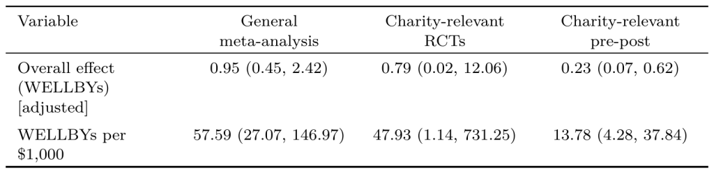
Note. Parentheses represent 95% confidence intervals.
Table 16: StrongMinds’ cost-effectiveness according to the different sources of evidence.
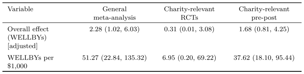
Note. Parentheses represent 95% confidence intervals.
Figure 11: Cost-effectiveness of the different charities based on different weightings between the sources of evidence.
Note. Dotted line is the WBp1k for the charity according to the overall effect averaged across the weights we give to the general evidence, the charity-related RCTs, and the charity M&E pre-post. We cannot represent the sensitivity of the weighting between three sources in this graph. Hence, the solid line is WBp1k across different weights given to the charity-related RCTs (on the left) or the charity M&E pre-post data (on the right) compared to the general meta-analysis (GMA). Dashed line is WBp1k of GiveDirectly. Top row is Friendship Bench, bottom row is StrongMinds.
8. Cost and cost-effectiveness
8.1 Friendship Bench
Based on their 2023 annual report and information communicated to us, we calculate that it costs = $3,530,397 / 214,020 (the number of clients who attended at least 1 session) = $16.50 for Friendship Bench to treat a person. We summarise cost-effectiveness results for Friendship Bench in Table 17.
Table 17: Friendship Bench cost-effectiveness.
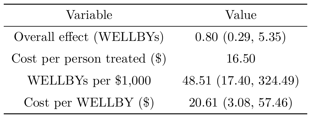
Note. Parentheses are 95% confidence intervals.
8.2 StrongMinds
In their 2023 Q4 report, StrongMinds reported treating 239,672 clients (i.e., who attended at least one session) for overall expenses of $9,789,291. Hence, the cost per person treated in 2023 was $41. Note that the cost to treat from StrongMinds has been steadily declining over timeThe costs per person treated for StrongMinds was $122 in 2018, $124 in 2019, $361 in 2020, $122 in 2021, $74 in 2022, and $41 in 2023. This is likely to decline further as the 2024 Q1 reportshows a cost per person treated of $31.. We then inflated the costs to $44.56 dollars (a downwards adjustment on the cost-effectiveness) based on inferences and calculations about the counterfactual of how many of StrongMinds’ partners would have treated patients for mental issues even without partnership with StrongMinds (see Appendix N for more detail). We summarise the cost-effectiveness of StrongMinds in Table 18 below.
Table 18: StrongMinds cost-effectiveness.
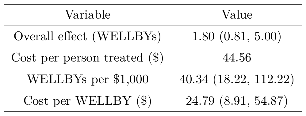
Note. Parentheses are 95% confidence intervals.
9. Confidence
In this section we discuss the factors that influence our confidence in our cost-effectiveness estimate (i.e., how confident we are that our analysis has produced the ‘true’ cost-effectiveness estimate of the charities). These factors are depth of evaluation (Section 9.1), quality of evidence (Section 9.2), sensitivity and robustness (Section 9.3), site visits (Section 9.4), and major outstanding uncertainties (Section 9.5).
9.1 Depth of evaluation
The depth of our analysis is based on a combination of how extensively we
have reviewed the literature and how comprehensive our analysis is. We use three depth ratings
in our work
.
Our psychotherapy analysis is the most in-depth analysis we have performed. Previously we said
this is a ‘moderate-to-in-depth’ report, we now think it is ‘high’
depth. Namely, we believe we have reviewed most or all of the relevant available evidence on
the topic, and we have completed nearly all (e.g., 90%+) of the analyses we think are useful.
However, a deep analysis should not be understood as one with no/low uncertainty. Like every cost-effectiveness, there are a few parameters that could alter the results substantially. This could be because the results are based on weak data (e.g., spillovers) or uncertain modelling (e.g., decay). We address the robustness of our findings to these factors in Section 9.3.
9.2 Quality of evidence using GRADE
Our method for evaluating the quality of evidence is based on stringent GRADE-adapted criteria. We discuss our methodology in Section 2.6.1. Below, we discuss our overall quality of evidence ratings for Friendship Bench and StrongMinds, and we also summarise the ratings for every source of evidence.
We think the quality of evidence for StrongMinds is low to moderate. This is because the general evidence for psychotherapy is moderate, and the Baird et al. RCT is low. Although the M&E pre-post data is very low (because it is not an RCT), its lower weight means it has a smaller influence on the overall evidence quality.
We think the quality of evidence for Friendship Bench is low to moderate. The general evidence is moderate, and the Friendship Bench RCT evidence is low to moderate. Although the M&E pre-post data is very low (because it is not an RCT), its lower weight means it has a smaller influence on the overall evidence quality.
The quality of evidence for the spillovers is very low. We take this into account for our overall assessment.
Table 19 shows all the inputs to our GRADE assessment with high quality (no concerns) ratings given in green, moderate (some concerns) in yellow, and low quality (major concerns) in red. The bottom rows also show how much of a role the spillovers play and how much weight the sources get.
See Appendix J for a more detailed account of the inputs into our assessment of quality.
Table 19: Quality of evidence summary.
|
Evidence sources |
Household Spillovers |
General evidence (as prior for FB and SM) |
FB RCTs |
FB M&E |
SM RCTs (Baird et al.) |
SM M&E |
|
Study design |
4 RCTs + 5 observational studies + 2 natural experiments |
RCTs |
RCTs |
pre-post |
RCT |
pre-post |
|
Risk of bias |
Barker et al. and Bryant et al. are 'some concerns'. The other studies are not evaluated. |
After removing high RoB, 57% are some concern, and 43% are low |
Haas et al. and Bengtson et al. are 'some concerns'. Chibanda et al. and Simms et al. are 'high' risk of bias. |
Not assessed. |
Baird et al. is 'some concerns' |
Not assessed. |
|
Imprecision (before adjustments) |
We are very uncertain about the estimates. They are based on meta-analytic ratios and pathways across two different methods. |
N = 25363, O = 68443, k = 84, m = 250 Initial effect (SDs): 0.59 (95% CI: 0.49, 0.69) Decay over time (SDs per year): -0.17 (95% CI: -0.26, -0.08) Total effect (SD-years): 1.02 (0.58, 2.30) |
N = 2011, O = 7377, k = 4, m = 15 Initial effect (SDs): 0.53 (95% CI: 0.04, 1.01) Decay over time (SDs per year): -0.16 (95% CI: -0.49, 0.17) Total effect (SD-years): 0.86 (0.02, 12.91) |
N = 2011, O = 7377, k = 4, m = 15 Initial effect (SDs): 0.12 (0.04, 0.19) (duration was imputed from GMA) Total effect (SD-years): 0.20 (0.07, 0.50) |
N = 1896, O = 7125, k = 1, m = 6 Initial effect (SDs): 0.10 (95% CI: 0.01, 0.19) Decay over time (SDs per year): -0.07 (95% CI: -0.13, 0.00) Total effect (SD-years): 0.07 (0.00, 0.71) |
N = 1896, O = 7125, k = 1, m = 6 Initial effect (SDs): 0.79 (0.74, 0.84) (duration was imputed from GMA) Total effect (SD-years): 1.38 (0.86, 2.96) |
|
Inconsistency (heterogeneity) |
Meta-analysis (12%) and pathways analyses (21%) suggest different ratios. We take the average. |
tau2 = 0.15 |
tau2 = 0.17 |
No comparison possible |
No comparison possible |
No comparison possible |
|
Indirectness (relatedness) |
Each study looks at different household members |
LMICs. We adjusted for as many characteristics as we could. We are still uncertain about the low dosage for Friendship Bench (see Section 5.2). |
Generally very similar context but some differences. Adjusted for difference in dosage. |
Direct |
BRAC delivering to teenagers in Uganda. Applied adjustments but we are still uncertain about the relevance of this study (see Section 7.3). |
Direct |
|
Publication bias |
Unclear, probably low because the studies are not directly investigating spillovers, but happen to report results for household members). |
Adjustment of 0.69 |
Adjustment of 0.92 because one of the four studies was not pre-registered. |
N/A |
Pre-registered and working report. |
N/A |
|
Source overall GRADE assessment |
Very Low |
Moderate |
Low to Moderate |
Very Low |
Low |
Very Low |
|
Household spillover contribution to overall effect (according to the source) |
N/A |
Friendship Bench: 32% StrongMinds: 38% |
32% |
32% |
38% |
38% |
|
Contribution of the source to the overall effect |
N/A |
Friendship Bench: 50% StrongMinds: 64% |
37% |
12% |
20% |
16% |
Note. Friendship Bench (FB), StrongMinds (SM), and general meta-analysis (GMA)
9.3 Sensitivity analysis and robustness
We present a sensitivity analysis to different plausible analytical choices. This serves two roles (Sections 9.3.1 to 9.3.3). One, to see how sensitive the analysis is to certain choices. Two, to see how robust the cost-effectiveness of the charities is to different choices. We also briefly discuss sensitivity to excluding outliers and high risk of bias studies (Section 9.3.4).
9.3.1 General method
We consider ‘plausible’ alternatives to our present analysisFor example, we do not show the results of picking the most stringent publication bias correction method just for the sake of showing the technical possibility. This is because we do not think choosing any one publication bias model is as justified as taking an average of them. . Although note that we erred on the side of inclusiveness, meaning we are not convinced all of these alternatives we present are plausible. In the tables below we present how plausible we think the different analyses are. Our best guess and the analysis we consider the most plausible is the one we presented in this report. If a reader believes one of these alternative analyses are more plausible, this would allow them to see what the results would be.
The alternative analyses we consider are:
- Focusing on the most or least cost-effective of the three sources of evidence (currently we weight them).
- Using the higher or lower value for spillovers (currently we use an average of the two).
- Using the most favourable dosage adjustment identified (i.e., no adjustment) or using the most stringent dosage adjustment identified (i.e., a simple linear adjustment). We currently use a moderate to stringent adjustment.
- Completely using the longterm follow-ups or completely removing the longterm follow-up (currently we use an upward time adjustment that represents giving 50% of the influence to a model with, and 50% of the influence to a model without, the long term follow-ups).
- Using no cost adjustment or a more stringent cost adjustment for counterfactuals for StrongMinds (currently we use a moderate adjustment based on information from StrongMinds).
- An analysis with all the favourable, or all the unfavourable, alternative analysis choices.
We think one important criteria for cost-effectiveness is whether an intervention is more (i.e., robust) or less (i.e., not robust) cost-effective than GiveDirectly cash transfersCash transfers are a common reference point in charity evaluations (GiveWell, 2018), and are also used as a benchmark when experimentally comparing the cost-effectiveness of interventions (e.g., McIntosh & Zeitlin, 2022) . To give some context to the robustness checks, we compare the alternative results to a few different reference points:
- Is it higher than the cost-effectiveness of GiveDirectly, which is 7.55 WBp1kNote that these are values of GiveDirectly at time of writing this report. This is also dependent on our current conversion ratio from SD-years to WELLBYs, currently at 2:1. This could change over time and we recommend interested readers consult our charities comparisons page on our website for up to date comparisons.?
- Is it higher than 20 WBp1k? We ask this because the cost-effectiveness of GiveDirectly might change in future analyses, and because we have some uncertainty around our analyses of psychotherapy and cash transfers, we want to test our charity evaluations against a larger buffer than the cost-effectiveness of GiveDirectly. 20 WBp1k represents ~2.6x the cost-effectiveness of GiveDirectly.
For simplicity, we consider our estimate of the cost-effectiveness of a charity to be robust if it does not go below 20 WBp1k with alternative analysis choices. We consider it is somewhat robust if a plausible alternative analysis suggests a cost-effectiveness below 20 WBp1k but at or above 7.55 WBp1k. We consider our analysis is not robust if a plausible alternative analysis suggests a cost-effectiveness below 7.55 WBp1k. However, this is another element of our analysis that we have not finalised. We think we could reasonably change the thresholds we use and our description of what constitutes robustness. We summarise the results for the charities in the subsections below. For more detail see Appendix O.
9.3.2 Friendship Bench
Friendship Bench’s cost-effectiveness is robust (i.e., above 20 WBp1k) to each individual unfavourable alternative choice on its own, except putting 100% of the weight on the pre-post data, the least cost-effective evidence source. This reduces the cost-effectiveness to 14 WBp1k (1.8x cash transfers).
When combining all the unfavourable alternative choices, the cost-effectiveness is 17 WBp1k (if we use our set weights for the different sources of evidence), and 13 WBp1k if we 100% of the weight on the pre-post data. The most optimistic individual analytical choice is using a more favourable dosage adjustment, resulting in 129 WBp1k (or 233 WBp1k when all favourable choices are combined). We do not consider these alternative choices as highly plausible.
The cost-effectiveness of Friendship Bench is most sensitive to the dosage adjustment selected and to – to some extent – to the influence given to the long term follow-ups and the weights between the sources of evidence.
The results for Friendship Bench are summarised in Table 20.
Table 20: Sensitivity analysis for Friendship Bench.
|
Robustness check |
WBp1k |
Adjustment |
Higher than 20 WBp1k? |
Higher than 1x GD (7.55 WBp1k)? |
Plausibility |
|
Current estimate |
49 |
- |
yes |
yes |
High |
|
100% of weight on lowest source (charity pre-post) |
14 |
0.28 |
no |
yes |
Low |
|
100% of weight on highest source (general meta-analysis) |
58 |
1.19 |
yes |
yes |
Low |
|
Longterm follow-ups: Fully remove |
38 |
0.79 |
yes |
yes |
Moderate |
|
Longterm follow-ups: Fully include |
60 |
1.23 |
yes |
yes |
Moderate |
|
Dosage adjustment: Most stringent |
23 |
0.47 |
yes |
yes |
Low-to-moderate |
|
Dosage adjustment: Most favourable |
129 |
2.66 |
yes |
yes |
Low-to-moderate |
|
Spillover ratio: Lower estimate |
44 |
0.91 |
yes |
yes |
Low |
|
Spillover ratio: Higher estimate |
53 |
1.09 |
yes |
yes |
High |
|
All unfavourable (only lowest source) |
13 |
0.26 |
no |
yes |
Very low |
|
All unfavourable (using our weights between the sources) |
17 |
0.35 |
no |
yes |
Very low |
|
All favourable (only highest source) |
233 |
4.80 |
yes |
yes |
Very low |
|
All favourable (using our weights between the sources) |
171 |
3.53 |
yes |
yes |
Very low |
9.3.3 StrongMinds
StrongMinds’ cost-effectiveness is robust (i.e., above 20 WBp1k) to each individual unfavourable alternative choice on its own, except putting 100% of the weight on Baird et al. (2024), the least cost-effective evidence source. Even when taking on this pessimistic view, this reduces the cost-effectiveness to 6.95 WBp1k (just below, but close to cash transfers).
Combining all the unfavourable alternative choices results in 19 WBp1k if we use our set weights for the different sources of evidence (and 4 WBp1k if we 100% of the weight on Baird et al.). The most optimistic individual analytical choice is using a more favourable duration of the effects, resulting in 58 WBp1k (or 97 WBp1k when all favourable choices are combined). We do not consider these alternative choices as highly plausible.
The cost-effectiveness of StrongMinds is most sensitive to the weight given to the different sources of evidence and to the influence given to the longterm follow-ups.
The results for StrongMinds are summarised in Table 21.
Table 21: Sensitivity analysis for StrongMinds
|
Robustness check |
WBp1k |
Adjustment |
Higher than 20 WBp1k? |
Higher than 1x GD (7.55 WBp1k)? |
Plausibility |
|
Current estimate |
40 |
- |
yes |
yes |
High |
|
100% of weight on lowest source (charity RCT: Baird et al.) |
7 |
0.17 |
no |
no |
Low |
|
100% of weight on highest source (general meta-analysis) |
51 |
1.27 |
yes |
yes |
Low |
|
Longterm follow-ups: Fully remove |
29 |
0.71 |
yes |
yes |
Moderate |
|
Longterm follow-ups: Fully include |
58 |
1.45 |
yes |
yes |
Moderate |
|
Dosage adjustment: Most stringent |
36 |
0.88 |
yes |
yes |
Low-to-moderate |
|
Dosage adjustment: Most favourable |
44 |
1.10 |
yes |
yes |
Low-to-moderate |
|
Spillover ratio: Lower estimate |
36 |
0.90 |
yes |
yes |
Low |
|
Spillover ratio: Higher estimate |
45 |
1.10 |
yes |
yes |
High |
|
Cost adjustment: Assume more stringent counterfactual |
34 |
0.83 |
yes |
yes |
Moderate |
|
Cost adjustment: No adjustment |
44 |
1.09 |
yes |
yes |
Moderate |
|
All unfavourable (only lowest source) |
4 |
0.09 |
no |
no |
Very low |
|
All unfavourable (using our weights between the sources) |
19 |
0.48 |
no |
yes |
Very low |
|
All favourable (only highest source) |
97 |
2.41 |
yes |
yes |
Very low |
|
All favourable (using our weights between the sources) |
77 |
1.90 |
yes |
yes |
Very low |
9.3.4 Sensitivity to excluding outliers and high risk of bias effect sizes
We believe that excluding outliers and high risk of bias effect sizes is the right analytical choice. The effects of psychotherapy and the cost-effectiveness of the charities are higher if we include these effect sizes (summarised in Table 22)That is despite a harsher publication bias adjustment, but this is due to some correction models overcorrecting, likely because of the enormous amount of heterogeneity (Tau2 in the table) if we do not exclude outlier studies. . For more details, see Appendix P.
In Appendix P4 we consider different ways of running the analysis with only low risk of bias studies. We did not consider this our main analysis because: this loses a lot of information, not all our moderators of interest (as per Appendix G2) can be well run, a study can be considered at more risk than ‘low’ as long as one subdomain is not considered ‘low’ risk (which could be stringent), the results are not very sensitive to this type of analysis, and cash transfers (our typical comparison point) do not have low risk of bias studies. The most severe way reduces the cost-effectiveness (StrongMinds: 30 WBp1k, Friendship Bench: 48 WBp1k) – but this seems to be due to a less reliable moderator analysis which we do not think is appropriate (see Appendix P4 for more detail), while the least severe way increases the cost-effectiveness (StrongMinds: 46 WBp1k, Friendship Bench: 56 WBp1k).
Table 22: Summary of sensitivity to excluding outliers and high risk of bias effect sizes.
|
Analysis |
Data |
General: Initial effect (SDs) |
General: Decay (SD change per year) |
General: Total effect (SD-years) |
Time adjustment |
Publication bias adjustment |
Total effect adjusted for time and publication bias (WELLBYs) |
FB: Overall effect (WELLBYs) |
SM: Overall effect (WELLBYs) |
FB: WBp1k |
SM: WBp1k |
Tau2 |
|
Main analysis (exclude outliers and high risk of bias) |
N = 25363, O = 68443, k = 84, m = 250 |
0.59 (0.49, 0.69) |
-0.17 (-0.26, -0.08) |
2.05 (1.16, 4.60) |
1.54 |
0.69 |
2.18 (1.23, 4.89) |
0.80 (0.29, 5.35) |
1.80 (0.81, 5.00) |
48.51 (17.40, 324.49) |
40.34 (18.22, 112.22) |
0.15 |
|
Include outliers but exclude high risk of bias |
N = 25943, O = 71091, k = 93, m = 290 |
0.82 (0.58, 1.07) |
-0.15 (-0.25, -0.06) |
4.44 (1.88, 13.47) |
1.44 |
0.38 |
2.45 (1.04, 7.44) |
0.75 (0.22, 5.37) |
1.86 (0.69, 6.52) |
45.21 (13.11, 325.48) |
41.81 (15.58, 146.34) |
1.06 |
|
Include outliers and include high risk of bias |
N = 31914, O = 83867, k = 127, m = 361 |
0.93 (0.72, 1.14) |
-0.15 (-0.25, -0.06) |
5.60 (2.77, 15.65) |
1.42 |
0.55 |
4.40 (2.18, 12.31) |
1.01 (0.36, 6.05) |
2.81 (1.16, 9.05) |
61.11 (21.61, 366.97) |
63.14 (26.07, 203.19) |
1.06 |
|
Exclude outliers but include high risk of bias |
N = 30775, O = 80181, k = 111, m = 306 |
0.63 (0.54, 0.72) |
-0.18 (-0.26, -0.09) |
2.24 (1.35, 4.56) |
1.53 |
0.71 |
2.42 (1.46, 4.93) |
0.85 (0.33, 5.34) |
1.88 (0.89, 4.86) |
51.26 (19.71, 324.00) |
42.10 (20.00, 109.13) |
0.15 |
Note. Friendship Bench (FB). StrongMinds (SM).
9.4 Site visits
Our director, Michael Plant, undertook two, day-long site visits to Friendship Bench in Zimbabwe and StrongMinds in Uganda. These visits increased our confidence that these are organisations that seem to be reasonably well functioning and to be making discernable impacts on people’s lives. We went in with a “trust, but verify” perspective: we expect these organisations and their staff are well-intentioned, but this did not mean they were highly cost-effective, so we wanted to understand the programmes better and look for any sources of concern. As discussed in more detail in the reports linked above, Michael came away pleasantly reassured. We do not put any weight on this numerically in this analysis, nor are we sure how we would do so. Michael came away thinking these organisations are doing useful, professional, and effective work.
Note that this does not tell us much, if anything, about comparative cost-effectiveness, and it was only a snapshot. Two organisations could be professionally operated but radically differ in cost-effectiveness based on what they do. If the organisations had seemed poorly run, we would have considered a downward adjustment and/or further investigation before making a recommendation.
9.5 Major outstanding uncertainties
Friendship Bench: We are still uncertain because of the very low attendance (dosage) of the Friendship Bench programme. We discuss this, and how it is not implausible that few sessions could still have an impact, in Section 5.2.4 and at length in Appendix H. We are also uncertain about the fact that the M&E pre-post data has lower results than the other two sources of evidence (which we discuss in Section 7.2). We have discussed this with Friendship Bench, and they inform us that they have planned future external monitoring and evaluating of their programme.
StrongMinds: We are still uncertain because the only RCT of the StrongMinds programme (Baird et al., 2024) is only partially relevant and shows a very low cost-effectiveness. We discuss this – notably the lack of relevance – in Sections 3.2.2 and 7.3, and at length in Appendix L. We have discussed this with StrongMinds and a more relevant RCT is in the works.
For both charities, we did our best to provide appropriate and informed weights between the different evidence sources. However, there is no precedent or standard way of assigning these weights. There remains a large element of subjectiveness in this process.
10. Conclusion
Overall, we conclude both charities are cost-effective at improving global wellbeing by providing important treatment to people with common mental disorders in different parts of SSA. These are the most cost-effective and well evidenced charities we have evaluated to date. We summarise information about the two charities in Table 23, below. See our website for more up to date information on the different charities we have evaluated.
Table 23: Summary of assessment of Friendship Bench and StrongMinds.
|
Friendship Bench |
StrongMinds |
|
|
Overall effect |
0.80 WELLBYs |
1.80 WELLBYs |
|
Cost per person |
$16.50 |
$44.56 |
|
Cost-effectiveness |
49 WBp1k (or $21 per WELLBY). |
40 WBp1k (or $25 per WELLBY). |
|
Depth of analysis |
High. We believe we have reviewed most or all of the relevant available evidence on the topic, and we have completed nearly all (e.g., 90%+) of the analyses we think are useful. |
High. We believe we have reviewed most or all of the relevant available evidence on the topic, and we have completed nearly all (e.g., 90%+) of the analyses we think are useful. |
|
Quality of evidence |
Overall: Low to moderate. General meta-analysis of psychotherapy: moderate. 84 RCTs with low (43%) and some (57%) risk of bias (high risk of bias studies were removed). Some inconsistency in effects, limited relevance, and some publication bias. FB RCTs: low to moderate. 4 RCTs with some (50%) and high (50%) risk of bias. Mostly relevant. Imprecision and inconsistency are moderate. Relatively little concern about publication bias. FB M&E: very low. Very relevant, but small sample and synthetic control provides limited information. Potential for substantial risks of bias. |
Overall: Low to moderate. General meta-analysis of psychotherapy: moderate. 84 RCTs with low (43%) some (57%) risk of bias (high risk of bias studies were removed). Some inconsistency in effects, limited relevance, and some publication bias. SM RCT (Baird et al.): low. 1 RCT with some risk of bias. Issues with relevance (see outstanding uncertainty). Moderate imprecision. Major inconsistency (because cannot verify with one study). No concern about publication bias. SM M&E: very low. Very relevant, but synthetic control provides limited information. Potential for substantial risks of bias. |
|
Robustness |
Friendship Bench’s cost-effectiveness is robust (i.e., above 20 WBp1k) to each individual unfavourable alternative choice on its own, except putting 100% of the weight on the pre-post data, the least cost-effective evidence source. This reduces the cost-effectiveness to 14 WBp1k (1.8x cash transfers). |
StrongMinds’ cost-effectiveness is robust (i.e., above 20 WBp1k) to each individual unfavourable alternative choice on its own, except putting 100% of the weight on Baird et al. (2024), the least cost-effective evidence source. Even when taking on this pessimistic view, this reduces the cost-effectiveness to 6.95 WBp1k (just below, but close to cash transfers). |
|
Site visit |
We are reassured by our site visit. |
We are reassured by our site visit. |
|
Major outstanding uncertainties |
We are still uncertain because of the very low attendance (dosage) of the FB programme. We discuss this, and how it is not implausible that few sessions could still have an impact, at length in Section 5.2.3. |
We are still uncertain because the only RCT of the SM programme (Baird et al., 2024) is only partially relevant and shows a very low cost-effectiveness. We discuss this at length, notably the lack of relevance, in Section 7.3 |
Appendices
Appendix A: Different versions
We have produced different versions of this analysis of psychotherapy in LMICs over the years. We summarise the differences between the versions in the table below.
Table A1: Summary of the differences between versions.
|
Version 1 (2021) |
Version 2 (2022) |
Version 3 (2023) |
Version 3.5 (2024) – a brief intermediate update |
Version 4 (2024) |
|
|
Reference (url) |
(McGuire & Plant, 2021b; McGuire & Plant, 2021c; McGuire et al., 2022b) |
Current version |
|||
|
Cost-effectiveness (StrongMinds) |
26 WBp1k, $42 per WELLBY, 12x cash [SD to WELLBY conversion was not used then so we use 2.17 for this reporting] |
62 WBp1k, $16 per WELLBY, 8x cash [SD to WELLBY conversion was not used then so we use 2.17 for this reporting] |
30 WBp1k, $33 per WELLBY, 4x cash |
47 WBp1k, $21 per WELLBY, 6x cash |
40 WBp1k, $25 per WELLBY, 5.3x cash |
|
Cost-effectiveness (Friendship Bench) |
Not evaluated |
Not evaluated |
58 WBp1k, $17 per WELLBY, 7x cash |
53 WBp1k, $19 per WELLBY, 7x cash |
49 WBp1k, $21 per WELLBY, 6.4x cash |
|
Give Directly cash transfers cost-effectiveness (at time of writing of the reports) |
2 WBp1k, $500 per WELLBY [SD to WELLBY conversion was not used then so we use 2.17 for this reporting] |
8 WBp1k, $125 per WELLBY [SD to WELLBY conversion was not used then so we use 2.17 for this reporting] |
8 WBp1k, $125 per WELLBY |
8 WBp1k, $125 per WELLBY |
7.55 WBp1k, $132 per WELLBY |
|
Cost to treat |
StrongMinds: $170 |
StrongMinds: $170 |
StrongMinds: $63 |
StrongMinds: $43 |
StrongMinds: $45 |
|
SD to WELLBYs conversion ratio |
Not included |
Not included |
2.17 |
2.17 |
2.00 |
|
Spillover ratio |
Not included |
38% (was corrected from 53%) |
16% |
16% |
16% |
|
Quality factors for the meta-analysis of psychotherapy in LMICs |
Systematised (i.e., non-exhaustive) review and meta-analysis |
Systematised (i.e., non-exhaustive) review and meta-analysis |
Systematic review and meta-analysis (excluding underpowered studies N < 61) |
Systematic review and meta-analysis (no exclusion for power). With risk of bias analysis. |
Systematic review and meta-analysis (no exclusion for power).
With double risk of bias analysis. |
|
Sources of evidence and detail (StrongMinds) |
(1) General psychotherapy in LMICs meta-analysis |
(1) General psychotherapy in LMICs meta-analysis |
(1) General psychotherapy in LMICs meta-analysis |
(1) General psychotherapy in LMICs meta-analysis |
(1) General psychotherapy in LMICs meta-analysis |
|
Sources of evidence and detail (Friendship Bench) |
Not evaluated |
Not evaluated |
(1) General psychotherapy in LMICs meta-analysis |
(1) General psychotherapy in LMICs meta-analysis |
(1) General psychotherapy in LMICs meta-analysis |
|
Weighting of sources of evidence: Method |
Subjective weights |
Subjective weights |
Bayesian weights for statistical uncertainty |
Informed subjective weights using GRADE structure and Bayesian weights for statistical uncertainty |
Informed subjective weights using GRADE structure and Bayesian weights for statistical uncertainty |
|
Weighting of sources of evidence: Weights (StrongMinds)Note that changes in weights between Versions 3.5 and 4 – for both StrongMinds and Friendship Bench – are mainly driven by changes in statistical uncertainty which influence the weights of some researchers who formed their subjective weights by adjusting the statistical uncertainty weights based on Bayesian updating. |
Multipart weighting process which was subjective. See paper for more detail. |
Multipart weighting process which was subjective. See paper for more detail. |
(1) 84% |
(1) 58% |
(1) 64% |
|
Weighting of sources of evidence: Weights (Friendship Bench) |
Not evaluated |
Not evaluated |
(1) 94% |
(1) 42% |
(1) 50% |
|
General meta-analysis: Number of studies before exclusions |
38 |
38 |
84 |
128 |
127 |
|
General meta-analysis: Number of studies after exclusions |
38 |
38 |
74 |
72 |
84 |
|
Number of studies in common with current version (before exclusion) |
21 |
21 |
79 |
127 |
Current version |
|
Exclusion criteria |
None |
None |
Outliers (g > 2) |
Outliers (g > 2) and ‘high’ risk of bias studies |
Outliers (g > 2) and ‘high’ risk of bias studies |
|
Time adjustment (for very longterm follow-ups) |
Not included |
Not included |
1.64 |
1.59 |
1.54 |
|
Publication bias adjustment |
0.89 (11% discount) |
0.89 (11% discount) |
0.64 (36% discount) |
0.71 (29% discount) |
0.69 (31% discount) |
|
Range restriction adjustment |
Not included |
Not included |
0.91 (9% discount) |
0.91 (9% discount) |
0.91 (9% discount) |
|
Moderator adjustment (StrongMinds) |
Not included |
Not included |
0.58 (42% discount) [only for the general meta-analysis] |
0.78 (22% discount) [only for the general meta-analysis] |
0.79 (21% discount) [only for the general meta-analysis] |
|
Moderator adjustment (Friendship Bench) |
Not evaluated |
Not evaluated |
0.37 (63% discount) [includes the dosage adjustment] |
0.97 (3% discount) [only for the general meta-analysis] |
0.90 (10% discount) [only for the general meta-analysis] |
|
Dosage predictor (with only follow-up time as a covariate) |
Not evaluated |
Not evaluated |
0.04 (-0.15, 0.22) SDs per log session |
0.23 (0.01, 0.46) SDs per log session |
0.02 (-0.15, 0.20) SDs per log session 0.07 (-0.12, 0.25) SDs per log sessions [after removing study with 32 intended sessions] |
|
Dosage adjustment (StrongMinds) |
Not included |
Not included |
Included in moderator adjustment |
(1) 0.94 (6% discount) |
(1) 0.90 (10% discount) |
|
Dosage adjustment (Friendship Bench) |
Not evaluated |
Not evaluated |
Included in moderator adjustment |
(1) 0.33 (67% discount) |
(1) 0.36 (64% discount) |
Appendix B: Systematic review and effect sizes
Here we present both our general methodology for extracting effect sizes as well as the data and results from our systematic review of psychotherapy in LMICs. This data is then used to predict effects for Friendship Bench and StrongMinds, and forms one of the data sources we used in our evaluations.
B1. Protocol
We pre-registered the methodology for our systematic review and our meta-analysis on PROSPERO (CRD42023431154). For more detail, including our pre-registered search strings, see this document. This document was updated to clarify our inclusion criteria once we had started to review papers and then our analysis choices as we conducted initial analysis and initial version of this report. Note that our analysis goes beyond the typical academic review and meta-analysis – especially in the charity sections – so we could not predict all our modelling choices. Some of our general methodology can be seen in our website methodology pages and in our previous analyses. Overall, we aimed to make the most rigorous choices despite there being many areas of our analysis where we could not follow clear precedented guidelines because such guidelines do not exist.
B2. Results of the systematic review
The results of our systematic review are summarised in Figure B1.
Figure B1: PRISMA.
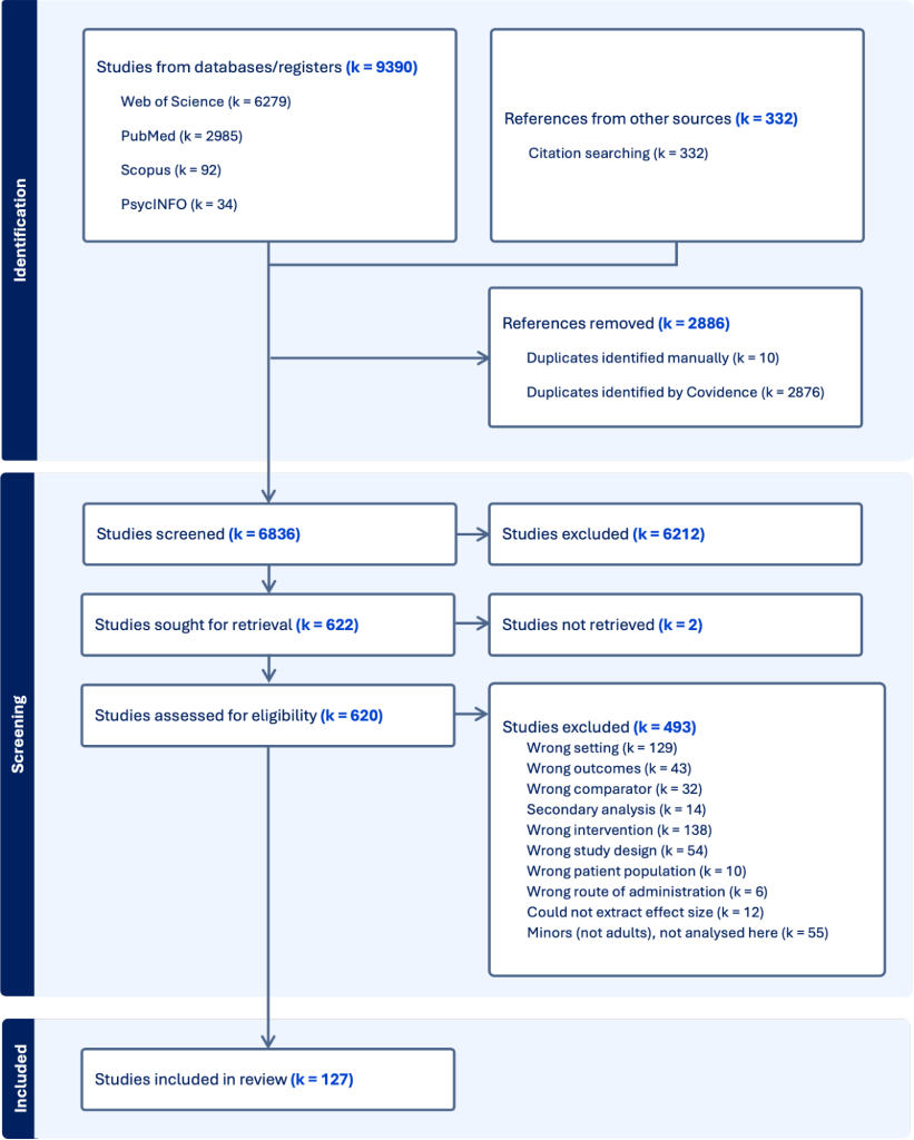
In sum, we have found and extracted results for 127 papers. Note that a ‘study’ in the graph refers to a paper. However, not each paper corresponds to one intervention, as sometimes different papers report on the same intervention (for different follow-ups, for example) or a paper might report on two interventions Bass et al. (2006) is a follow-up of Bolton et al. (2003). Fard et al.’s (2018) sample was split between those who did a pre-test at baseline and those who did not. Namasaba et al. (2022) reported on one intervention for caregivers of children with disability in the home, and one intervention for caregivers of children with disability in schools. The Health Activity Program was reported on by multiple papers (Patel et al., 2017; Weobong et al., 2017; Bhat et al., 2022). The Thinking Healthy Programme Peer-Delivered (THPP) in India was reported on by multiple papers (Fuhr et al., 2019; Bhat et al., 2022). The Buenaventura and Quibdo interventions were both reported on in multiple papers by Bonnilla-Escobar et al. (2018, 2023a, 2023b). Weiss et al. (2015) reported both a CETA and a CPT intervention.. Our analysis includes 127 interventions. Henceforth, by ‘study’, we will mean ‘intervention’ and not ‘paper’.
B3. Data extraction and effect sizes
In line with previous meta-analyses of depression (see Section 1) we standardised the effect sizes using standardised mean difference (Harrer et al., 2021). First, we calculated Cohen’s d using either the means and standard deviations of the control and treatment groups, or using the mean difference and standard error of the mean difference (Lakens, 2013). Then we converted Cohen’s d to Hedges’ g because it is a less biased estimate, especially for small sample sizes (Hedges & Olkin, 1985; Lakens, 2013). We calculated the standard error of the effect size based on Cohen’s d (Harrer et al., 2021) because using Hedges’ g will underestimate the standard error (Hedges et al., 2023).
For many interventions we extracted more than one effect size, because the intervention had multiple outcomes that fit our inclusion criteria and multiple follow-ups. This resulted in k = 127 interventions with m = 361 effect sizes, with O = 83,867 observations from N = 31,914 unique participants.
The vast majority of outcomes we found were continuous (m = 358, 99%), confirming the choice for Cohen’s d and Hedges’ g. For dichotomous outcomes (m = 3, 1%), we calculated an odds ratio, which we then converted to Cohen’s d using the Cox and Snell method, and then we converted from Cohen’s d to Hedges’ g. Cochrane guidelines (Higgins et al., 2023, Section 10.6) only mention the Hasselblad and Hedges method, but as a “simple approach”. Cochrane guidelines cite Anzures-Cabrera et al. (2011) but do not mention that the authors compare both the Hasselblad and Hedges and the Cox and Snell methods, and found both to perform similarly. According to Sánchez-Meca et al. (2003) and our unpublished simulations, the Cox and Snell method performs better which is why we select it.
Many authors do not report their results in a consistent manner. Sometimes the means and standard deviations of the control and treatment groups are presented, other times it is a mean difference, and other times it is a mean difference that is adjusted for baseline characteristics or an imbalance between treatment and control groups. Furthermore, authors sometimes apply different adjustments for their effects. We contacted authors when results were unclear or missing. Most authors did not respond, but we are grateful for the responses we receivedWe thank Dr Baranov, Dr Haushofer, Dr Weiss, Dr Sanborn, Dr Gallis, Dr Turner, Dr Lund, Dr Shaw, and Dr Patel. .
Following guidelines from Cochrane (Higgins et al., 2023, Section 6.3) we use adjusted values when the authors adjust for baseline scores (in case of a potential imbalance), clustering (notably for cluster RCTs), other justifiable adjustments, and when the unadjusted values are not available. “Other justifiable adjustments” is due to some vagueness from Point 2 of the Cochrane guidelines (Higgins et al., 2023, Section 6.3): “For specific analyses of randomized trials: there may be other reasons to extract effect estimates directly, such as when analyses have been performed to adjust for variables used in stratified randomization or minimization, or when analysis of covariance has been used to adjust for baseline measures of an outcome. Other examples of sophisticated analyses include those undertaken to reduce risk of bias, to handle missing data or to estimate a ‘per-protocol’ effect using instrumental variables analysis (see also Chapter 8)”. We reached out to Cochrane guideline authors and were instructed that whatever type of adjustment we included, we should be consistent throughout the analysis. We did not use adjustments when they only involved baseline covariates that were not the baseline scores on the outcome measure (e.g., adjusting only for education). However, if there was an adjustment for baseline outcome scores or clustering, and we could not have these without other covariates, we included adjustments from other covariates that the authors had added.
There were no adjustments for m = 233 (65%) of effect sizes, adjustments for baseline outcome scores for m = 57 (16%) effect sizes, adjustments for clustering for 19 (5%) effect sizes, adjustments for both baseline outcome scores and clustering for m = 41 (11%) effect sizes, and miscellaneous adjustments we had no choice to extract for m = 11 (3%) effect sizes.
Literature suggests that correcting for baseline imbalance, especially in the case of the outcome of interest to us, is important for accurate results (Trowman et al., 2007; Senn, 2012; Riley et al., 2013; Egbewale et al., 2014; Kahan et al., 2014; Holmberg et al., 2022; Pirondini et al., 2022). For the m = 263 (73%) effect sizes where there was no adjustment for baseline scores on the outcome of interest from the authors, we tested (using an independent t-test) for baseline imbalance between the treatment and control group on the outcome of interest when possible. If there was a significant baseline imbalance we used a difference-in-difference adjustment to the mean difference, thereby adjusting the effect size. This was applied to 18 (5%) effect sizes. Based on the literature, this is the typical approach used (Trowman et al., 2007; Morris, 2008; Villa, 2016; Hedges et al., 2023). There is not a lot of research (Morris, 2008; Hedges et al., 2023) about what to do with the pooled SD (the denominator in calculating Cohen's d). We follow Morris’s (2008) recommendation that the best method is to use the SD pooled at baseline.
Adjustments for clustering are important otherwise there is unaccounted dependency between the results of the different participants. There were 19 (5%) effect sizes from 5 cluster RCTs (4% of all interventions) without adjustments for clustering. There is a correction that we can apply to these studies to approximate the adjustment that would have occurred if results had been adjusted for clustering by the authors. This is based on reducing the effective sample size which will reduce the effect size and increase the standard error of the effect size, the adjustment is calculated as 1 + (M-1) * ICC, where M is the average size of the clusters in participants (White & Thomas, 2005; Higgins et al., 2023; Section 23.1.4). This requires having the ICC for the different studies we would like to adjust, however, authors rarely report this information. Instead, we rely on the ICC reported in other studies in our meta-analysis, and use the average of these, an ICC of 0.07.
There were 11 (9%) interventions that had one control group for multiple treatment arms. This would lead to double counting of the control group. Following guidelines (Harrer et al., 2021; Higgins et al., 2023, Section 23.3.4) we combine the multiple treatment groups to form only one pairwise comparison with the control group. These guidelines apply to extractions of means and SDs for the control and treatment group. However, there are many extractions where we only have the difference between the means and the standard error for this difference. This often happened because we extracted an adjusted effect; hence, we want to keep the influence of the adjustment in our combination. To do so, we apply the same formula used to combine the means to the mean difference, and the formula used to combine the SDs to the standard error of the mean difference.
In our meta-analysis, we prioritised extracting results from Intention-to-Treat (ITT) analyses wherever possible. ITT analysis includes all participants as originally assigned to the treatment or control group, regardless of whether they completed the treatment or followed the protocol. This approach helps to maintain the benefits of randomisation and reflects real-world implementation by addressing issues like non-compliance and dropouts. However, authors often do not clearly specify their analytical approach. In these cases, we classified the analysis as ITT, likely ITT (if patterns such as imputation for missing data or lack of attrition were observed), Treatment-on-the-Treated (ToT), or likely ToT. ToT focuses only on participants who adhered to their assigned treatment, providing insight into the effect on those who received the intervention as intended, but it can introduce bias due to excluding non-compliant participants. See Table B1 for a summary. The inclusion of some ToT or likely ToT results did not lead to an overestimate of the effects of psychotherapy, as we find in a meta-regression analysis that ToT (and likely ToT) effect sizes had, on average, non-significantly lower results by 0.21 (95% CI: -0.66, 0.24) SDs than results from ITT (or likely ITT) effect sizes.
Table B1: Distribution of ITT or ToT effect sizes in our data.
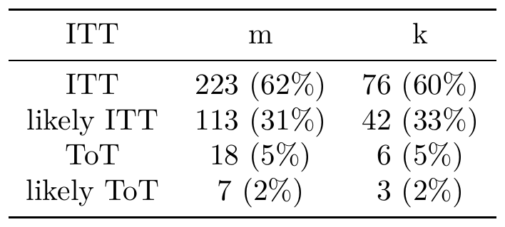
B4. Double-checking
We conducted multiple checks on our extraction to ensure our results were accurate. First we conducted preliminary checks by double checking outliers, negative effect sizes, long-term follow-ups, large studies, studies related to the charities we are evaluating, and we double checked whether we were using the right information when authors presented different results with different adjustments. Then, we conducted a thorough overall double check with two double-checkers who were not the initial extractors who checked every number we had extracted (this is the method used for our meta-analysis of cash transfers published in Nature Human Behaviour; McGuire et al., 2022a).
B5. Risk of bias analysis
In collaboration with academics from Oxford and Paris (see our Notes and Acknowledgements in the report), we conducted a Risk of Bias (RoB; Sterne et al., 2019) analysis. Since Version 3.5 we conducted a second round of risk of biasIn assessing the risk of bias in our review, we encountered discrepancies among reviewers regarding Domain 2, Part B, criterion 2.5B, which concerns non-adherence to the assigned intervention that could affect participants’ outcomes. The core issue was whether varying levels of session attendance in psychotherapy interventions should be considered non-adherence due to deviations arising from the trial context. After discussion, we determined that incomplete session attendance is a reasonable occurrence in psychotherapy studies, especially in low-resource settings, and typically reflects real-world conditions rather than trial-induced deviations. Therefore, we decided not to mark reduced session attendance as a bias under criterion 2.5B unless it was a direct result of the trial context or led to systematic exclusion of participants from the analysis. If participants attend fewer sessions, then the effect will be smaller. As long as the fewer sessions have not been caused by some deviation in the intervention (e.g., the researchers started barring some people from attending), this would not be a systematic overestimation of the effect of psychotherapy. analysis to check for and resolve potential mismatches in evaluations, which has changed the ratings of some studies.
This is the academically standard way of assessing if a study has flaws in its design or implementation which could ‘bias’ the result (downward or, more commonly, upwards). Assessing RoB is a sort of ‘due diligence’ for a systematic review and meta-analysis, one that is time consuming (but often, although not always, done for academic publications). A classic example of bias in a medical trial would be participants not being ‘blinded’ as to whether they receive the drug or a placebo.
Raters assess studies on five subdomains according to criteria set out by Cochrane (Sterne et al., 2019). For a study to be considered ‘low’ risk of bias, all five domains need to be rated as low. If at least one of the criteria is evaluated as ‘some concerns’, then the overall rating will be ‘some concerns’. If at least one of the criteria is evaluated as ‘high’ risk of bias, then the overall rating will be ‘high’. See Figure B2 and Table B2 for the results.
Figure B2: Risk of Bias distribution before any removals.
Table B2: Risk of Bias distribution before any removals.
Readers unfamiliar with RoB analysis should not assume that a ‘high’ risk of bias indicates that the study’s author(s) are corrupt or incompetent, only that they are reasons to doubt the results. Note that it may be difficult to conduct some studies in less biased ways depending on their context.
In our case, we assumed studies with high risk of bias are not as reliable and are likely to inflate the effect estimate. Hence, of our 127 interventions, we exclude 34 interventions (or 71 effect sizes) with ‘high’ risk of bias. Leaving us with 56 interventions rated as ‘some concern’ and 37 interventions with ‘low’ risk of bias (for a total of 93 interventions). See Section 9.3.4 and Appendix P for how much this influences the analysis (not much).
B6. Forest plots and references
Next, in Figures B3 to B12, we present forest plots of the effects sizes. Because there are 359 effect sizes, this is split across 10 figures. These are presented in alphabetical order of the intervention label, combined for each intervention-outcome combination (e.g., some interventions report results with two or more outcome measures), and then ordered according to the follow-up time in years from the end of the intervention (the number in parentheses). The dependencies of effect sizes (multiple effect sizes per outcomes and interventions), makes a simple order by magnitude of effect sizes seem more confusing to us. In Table B3 we present a list of references.
Figure B3: Forest plot of effect sizes (part 1).
Figure B4: Forest plot of effect sizes (part 2).
Figure B5: Forest plot of effect sizes (part 3).
Figure B6: Forest plot of effect sizes (part 4).
Figure B7: Forest plot of effect sizes (part 5).
Figure B8: Forest plot of effect sizes (part 6).
Figure B9: Forest plot of effect sizes (part 7).
Figure B10: Forest plot of effect sizes (part 8).
Figure B11: Forest plot of effect sizes (part 9).
Figure B12: Forest plot of effect sizes (part 10).
Table B3: References.
|
authors |
url |
|
Abbas et al. 2022 |
https://bmcpsychiatry.biomedcentral.com/articles/10.1186/s12888-022-03863-w |
|
Abbas et al. 2023 |
https://pubmed.ncbi.nlm.nih.gov/37491185/ |
|
Acarturk et al. 2015 |
https://pubmed.ncbi.nlm.nih.gov/25989952/ |
|
Acarturk et al. 2016 |
https://pubmed.ncbi.nlm.nih.gov/27353367/ |
|
Acarturk et al. 2022a |
https://bmcpsychiatry.biomedcentral.com/articles/10.1186/s12888-021-03645-w |
|
Adina et al. 2017 |
https://www.ijpsy.com/volumen17/num2/464.html |
|
Alagheband et al. 2019 |
https://www.tandfonline.com/doi/abs/10.1080/13674676.2018.1517254 |
|
Ali et al. 2003 |
https://psychotherapy.psychiatryonline.org/doi/10.1176/appi.psychotherapy.2003.57.3.324 |
|
Ara et al. 2023 |
https://link.springer.com/article/10.1007/s41811-023-00160-8 |
|
Asghari et al. 2016 |
https://www.ncbi.nlm.nih.gov/pmc/articles/PMC5198402/ |
|
Ayoughi et al. 2012 |
https://bmcpsychiatry.biomedcentral.com/articles/10.1186/1471-244X-12-14 |
|
Ayudhaya et al. 2020 |
https://www.ncbi.nlm.nih.gov/pmc/articles/PMC7753897/ |
|
Barker et al. 2022 |
https://www.aeaweb.org/articles?id=10.1257/aeri.20210612 |
|
Basirat et al. 2022 |
https://pubmed.ncbi.nlm.nih.gov/36029059/ |
|
Bass et al. 2006 |
https://www.cambridge.org/core/journals/the-british-journal-of-psychiatry/article/group-interpersonal-psychotherapy-for-depression-in-rural-uganda-6month-outcomes/34A03947B7B1F12CD5E364AD54B45626 |
|
Bass et al. 2013 |
https://www.nejm.org/doi/full/10.1056/nejmoa1211853 |
|
Bass et al. 2016 |
https://www.ghspjournal.org/content/4/3/452 |
|
Belay et al. 2022 |
https://link.springer.com/article/10.1007/s00520-021-06508-y |
|
Bhat et al. 2022 |
https://www.nber.org/papers/w30011 |
|
Bogdanov et al. 2021 |
https://www.cambridge.org/core/journals/global-mental-health/article/randomizedcontrolled-trial-of-communitybased-transdiagnostic-psychotherapy-for-veterans-and-internally-displaced-persons-in-ukraine/E5D56D4ABFD072D525D371F080F2BAF0 |
|
Bolton et al. 2003 |
https://jamanetwork.com/journals/jama/fullarticle/196766 |
|
Bolton et al. 2014 |
https://pubmed.ncbi.nlm.nih.gov/25551436/ |
|
Bolton et al. 2014b |
https://journals.plos.org/plosmedicine/article?id=10.1371/journal.pmed.1001757 |
|
Bonilla-Escobar et al. 2018 |
https://pubmed.ncbi.nlm.nih.gov/30532155/ |
|
Bonilla-Escobar et al. 2023b |
https://www.tandfonline.com/doi/full/10.1080/13623699.2023.2196500 |
|
Borji et al. 2017 |
https://www.ncbi.nlm.nih.gov/pmc/articles/PMC5980872/ |
|
Bryant et al. 2011 |
https://www.ncbi.nlm.nih.gov/pmc/articles/PMC3188775/ |
|
Bryant et al. 2017 |
https://journals.plos.org/plosmedicine/article?id=10.1371/journal.pmed.1002371 |
|
Bryant et al. 2022b |
https://www.cambridge.org/core/journals/epidemiology-and-psychiatric-sciences/article/twelvemonth-followup-of-a-randomised-clinical-trial-of-a-brief-group-psychological-intervention-for-common-mental-disorders-in-syrian-refugees-in-jordan/BC3F28C8057E2F87D86955C32C515C31 |
|
Chan et al. 2012 |
https://pubmed.ncbi.nlm.nih.gov/22840618/ |
|
Chibanda et al. 2016 |
https://jamanetwork.com/journals/jama/fullarticle/2594719 |
|
Chowdhary et al. 2016 |
https://pubmed.ncbi.nlm.nih.gov/26494875/ |
|
Dawson et al. 2016 |
https://bmcpsychiatry.biomedcentral.com/articles/10.1186/s12888-016-1117-x#Sec17 |
|
Demir & Ercan 2022 |
https://pubmed.ncbi.nlm.nih.gov/35332542/ |
|
Dereix-Calonge et al. 2019 |
https://psycnet.apa.org/record/2019-11045-001 |
|
Dowlatabadi et al. 2016 |
https://www.ncbi.nlm.nih.gov/pmc/articles/PMC4844485/ |
|
Esfandiari et al. 2020 |
https://pubmed.ncbi.nlm.nih.gov/32439135/ |
|
Ezegbe et al. 2019 |
https://pubmed.ncbi.nlm.nih.gov/30985642/ |
|
Fard et al. 2018 |
https://www.sciencedirect.com/science/article/pii/S1110569018301031 |
|
Fereydouni & Forstmeier 2022 |
https://pubmed.ncbi.nlm.nih.gov/35018526/ |
|
Foo et al. 2020 |
https://www.mdpi.com/1660-4601/17/17/6179 |
|
Fuhr et al. 2019 |
https://www.thelancet.com/journals/lanpsy/article/PIIS2215-0366(18)30466-8/fulltext |
|
Gao et al. 2010 |
https://www.sciencedirect.com/science/article/pii/S0020748910001045 |
|
Golshani et al. 2021 |
https://www.ncbi.nlm.nih.gov/pmc/articles/PMC8167953/ |
|
Greene et al. 2021 |
https://journals.plos.org/plosone/article?id=10.1371/journal.pone.0252982 |
|
Guo et al. 2016 |
https://pubmed.ncbi.nlm.nih.gov/27633932/ |
|
Gureje et al. 2019 |
https://pubmed.ncbi.nlm.nih.gov/30767826/ |
|
Haas et al. 2023 |
https://jamanetwork.com/journals/jamanetworkopen/fullarticle/2807191 |
|
Hamamci 2006 |
https://psycnet.apa.org/record/2006-08901-004 |
|
Hamdani et al. 2021 |
https://ijmhs.biomedcentral.com/articles/10.1186/s13033-020-00434-y |
|
Haushofer et al. 2023 |
https://www.nber.org/papers/w28106 |
|
Hemanny et al. 2020 |
https://pubmed.ncbi.nlm.nih.gov/31769377/ |
|
Hirani et al. 2010 |
https://ecommons.aku.edu/pakistan_fhs_son/112/ |
|
Husain et al. 2014 |
https://pubmed.ncbi.nlm.nih.gov/24676964/ |
|
Husain et al. 2023 |
https://bmcmedicine.biomedcentral.com/articles/10.1186/s12916-023-02983-8 |
|
Jalali et al. 2019c |
https://pubmed.ncbi.nlm.nih.gov/29938557/ |
|
Jordans et al. 2019 |
https://pubmed.ncbi.nlm.nih.gov/30678744/ |
|
Jordans et al. 2021 |
https://journals.plos.org/plosmedicine/article?id=10.1371/journal.pmed.1003621 |
|
Kaaya et al. 2022 |
https://journals.plos.org/plosmedicine/article?id=10.1371/journal.pmed.1004112 |
|
Karimi et al. 2019 |
https://www.tandfonline.com/doi/pdf/10.1080/01612840.2019.1609635 |
|
Khan et al. 2017b |
https://pubmed.ncbi.nlm.nih.gov/28689511/ |
|
Khoshbooii et al. 2021 |
https://www.ncbi.nlm.nih.gov/pmc/articles/PMC8303550/ |
|
Lenglet et al. 2018 |
https://bmjopen.bmj.com/content/8/8/e019794 |
|
Liu & Yang 2021 |
https://annals-general-psychiatry.biomedcentral.com/articles/10.1186/s12991-020-00320-4 |
|
Longchoopol et al. 2018 |
https://he02.tci-thaijo.org/index.php/PRIJNR/article/view/78778 |
|
Lund et al. 2020 |
https://www.sciencedirect.com/science/article/pii/S0005796719301524 |
|
Mahmoodi et al. 2020 |
https://www.cambridge.org/core/journals/behavioural-and-cognitive-psychotherapy/article/abs/comparison-between-cbt-focused-on-perfectionism-and-cbt-focused-on-emotion-regulation-for-individuals-with-depression-and-anxiety-disorders-and-dysfunctional-perfectionism-a-randomized-controlled-trial/77BC4F1A6EB62D5304E467BCA5383363 |
|
Majidzadeh et al. 2023 |
https://bmcpsychiatry.biomedcentral.com/articles/10.1186/s12888-023-04814-9 |
|
Mao et al. 2012 |
https://onlinelibrary.wiley.com/doi/10.1111/j.1744-6163.2012.00331.x |
|
Markkula et al. 2019 |
https://pubmed.ncbi.nlm.nih.gov/31391947/ |
|
Maselko et al. 2020 |
https://www.thelancet.com/journals/lanpsy/article/PIIS2215-0366(20)30258-3/fulltext |
|
Matsuzaka et al. 2017 |
https://www.ncbi.nlm.nih.gov/pmc/articles/PMC5480168/ |
|
Meffert et al. 2014 |
https://psycnet.apa.org/record/2011-08634-001 |
|
Meffert et al. 2021 |
https://journals.plos.org/plosmedicine/article?id=10.1371/journal.pmed.1003468 |
|
Mirtabar et al. 2020 |
https://pubmed.ncbi.nlm.nih.gov/32778009/ |
|
Mirzania et al. 2021 |
https://brieflands.com/articles/ijcm-112915 |
|
Mohammadpour et al. 2021 |
https://bmcpsychiatry.biomedcentral.com/articles/10.1186/s12888-021-03217-y |
|
Monfaredi et al. 2022 |
https://pubmed.ncbi.nlm.nih.gov/35148706/ |
|
Mukhtar 2011 |
https://www.sciencedirect.com/science/article/abs/pii/S1876201811000396?via%3Dihub |
|
Myers et al. 2022 |
https://www.thelancet.com/journals/lancet/article/PIIS0140-6736(22)01641-5/fulltext |
|
Naeem et al. 2011 |
https://pubmed.ncbi.nlm.nih.gov/21092353/ |
|
Naeem et al. 2015 |
https://www.sciencedirect.com/science/article/abs/pii/S0165032715000889 |
|
Namasaba et al. 2022 |
https://pubmed.ncbi.nlm.nih.gov/36579518/ |
|
Nikrahan et al. 2016 |
https://www.sciencedirect.com/science/article/pii/S0033318216000487 |
|
Nourisaeed et al. 2021 |
https://arya.mui.ac.ir/article_10785.html |
|
Onyishi et al. 2023 |
https://www.sciencedirect.com/science/article/pii/S175094672200157X |
|
Patel et al. 2017 |
https://www.thelancet.com/journals/lancet/article/PIIS0140-6736(16)31589-6/fulltext |
|
Petersen et al. 2014 |
https://pubmed.ncbi.nlm.nih.gov/24655769/ |
|
Pinjarkar et al. 2018 |
https://link.springer.com/article/10.1007/s41811-018-0025-x |
|
Qiu et al. 2013 |
https://pubmed.ncbi.nlm.nih.gov/23646866/ |
|
Rahimi et al. 2021 |
https://bmcpsychiatry.biomedcentral.com/articles/10.1186/s12888-021-03280-5 |
|
Rahman et al. 2008 |
https://www.thelancet.com/journals/lancet/article/PIIS0140-6736(08)61400-2/fulltext |
|
Rahman et al. 2016 |
https://pubmed.ncbi.nlm.nih.gov/27837602/ |
|
Rahman et al. 2019 |
https://pubmed.ncbi.nlm.nih.gov/30948286/ |
|
Raji Lahiji et al. 2022 |
https://pubmed.ncbi.nlm.nih.gov/35759049/ |
|
Raphi et al. 2021 |
https://bmcpsychiatry.biomedcentral.com/articles/10.1186/s12888-021-03600-9 |
|
Reddy & Omkarappa 2019 |
https://www.ncbi.nlm.nih.gov/pmc/articles/PMC6482762/ |
|
Robjant et al. 2019 |
https://pubmed.ncbi.nlm.nih.gov/31639529/ |
|
Safren et al. 2021 |
https://onlinelibrary.wiley.com/doi/10.1002/jia2.25823 |
|
Sangraula et al. 2020 |
https://www.ncbi.nlm.nih.gov/pmc/articles/PMC7264859/ |
|
Sapkota et al. 2020 |
https://journals.sagepub.com/doi/abs/10.1177/0886260520948151 |
|
Savari et al. 2021 |
https://link.springer.com/article/10.1007/s12671-020-01584-3 |
|
Seiiedi-Biarag et al. 2021 |
https://bmcpregnancychildbirth.biomedcentral.com/articles/10.1186/s12884-020-03502-w |
|
Shareh & Yazdanian 2023 |
https://pubmed.ncbi.nlm.nih.gov/36893401/ |
|
Shata et al. 2017 |
https://pubmed.ncbi.nlm.nih.gov/28469987/ |
|
Shaw et al. 2019 |
https://pubmed.ncbi.nlm.nih.gov/30035560/ |
|
Sikander et al. 2019 |
https://pubmed.ncbi.nlm.nih.gov/30686386/ |
|
Sinniah et al. 2017 |
https://pubmed.ncbi.nlm.nih.gov/28463716/ |
|
Soori et al. 2018 |
https://journals.sagepub.com/doi/10.1177/20533691221136309 |
|
Taghvaienia & Alamdari 2020 |
https://pubmed.ncbi.nlm.nih.gov/31552541/ |
|
Tshabalala & Visser 2011 |
https://journals.sagepub.com/doi/10.1177/008124631104100103 |
|
Wang et al. 2021 |
https://pubmed.ncbi.nlm.nih.gov/33812296/ |
|
Watt et al. 2017 |
https://pilotfeasibilitystudies.biomedcentral.com/articles/10.1186/s40814-017-0178-z |
|
Weiss et al. 2015 |
https://bmcpsychiatry.biomedcentral.com/articles/10.1186/s12888-015-0622-7 |
|
Weobong et al. 2017 |
https://journals.plos.org/plosmedicine/article?id=10.1371/journal.pmed.1002385 |
|
Wijesinghe et al. 2015 |
https://journals.plos.org/plosntds/article?id=10.1371/journal.pntd.0003989 |
|
Xie et al. 2017 |
https://www.tandfonline.com/doi/abs/10.1080/10503307.2017.1364444 |
|
Yator et al. 2022 |
https://psychiatryonline.org/doi/10.1176/appi.psychotherapy.20200050?url_ver=Z39.88-2003&rfr_id=ori:rid:crossref.org&rfr_dat=cr_pub%20%200pubmed |
|
Yuan et al. 2020 |
https://pubmed.ncbi.nlm.nih.gov/33118908/ |
|
Zahedian et al. 2021 |
https://bmcwomenshealth.biomedcentral.com/articles/10.1186/s12905-021-01258-9 |
|
Zang et al. 2013 |
https://bmcpsychiatry.biomedcentral.com/articles/10.1186/1471-244X-13-41 |
|
Zang et al. 2014 |
https://pubmed.ncbi.nlm.nih.gov/25927297/ |
|
Zemestani & Mozaffari 2020 |
https://pubmed.ncbi.nlm.nih.gov/32476482/ |
|
Zemestani & Nikoo 2019 |
https://pubmed.ncbi.nlm.nih.gov/30982086/ |
|
Zhao et al. 2018 |
https://onlinelibrary.wiley.com/doi/abs/10.1111/eip.12731 |
|
Zu et al. 2014 |
https://pubmed.ncbi.nlm.nih.gov/24140226/ |
|
Zuo et al. 2022 |
https://bmcpublichealth.biomedcentral.com/articles/10.1186/s12889-022-14631-6 |
Appendix C: Meta-analysis modelling
In this appendix we discuss the general meta-analysis methodology that we follow. We conduct our analysis in R and aim to follow accepted precedent guidelines about meta-analysis methodology when available (e.g., Harrer et al., 2021). In Appendix C2 we also provide details about the heterogeneity of our general meta-analysis of psychotherapy in LMICs. In Appendix C3 we discuss the multilevel modelling options of our general meta-analysis.
C1. Choosing a fixed or random effects model
The idea behind a meta-analysis is to pool effect sizes from multiple studies to get closer to the “true” population effect. The main modelling choice is between using a fixed effect (FE; or ‘common effect’) model or a random effects (RE) model.
A FE model assumes a homogeneous population, that all effect sizes share the same ‘true’ effect size, and that we do not want to generalise the results beyond the narrowly defined population (Borenstein et al., 2010; Harrer et al., 2021). For example, applying the FE assumptions to this analysis would mean that across all LMICs, all the different ways psychotherapy is implemented leads to the same effect.
In a RE model, the effect sizes are not expected to be sampled from a homogeneous population with a ‘true’ effect size, but from a population of ‘true’ effect sizes, where the overall pooled effect is the mean of this population (Harrer et al., 2021). Hence, a RE model expects and accounts for heterogeneity between the effect sizes due to all sorts of reasons beyond sampling error alone (e.g., different recipients, treatments, or measurement methods). It does so by estimating the heterogeneity with an algorithm and adding it to the weights of the different effect sizes. Typically, this leads to more accurate (and higher) estimates of the results’ uncertainty.
We expect (and find) high levels of heterogeneity in our data and our subject matter does not fit the conditions for a FE model; hence, we follow the guidelines and use a RE model. This is typical of this sort of literature (Harrer et al., 2021). A RE model incorporates and quantifies heterogeneity but it does not explain it; hence, we seek to do so with moderation analyses (Kriston, 2013; Higgins et al., 2023; see Appendices D and G).
C2. Assessing heterogeneity (variation between effect sizes)
Heterogeneity in a meta-analysis refers to the variability or differences between the effect sizes that is not due to chance (i.e., not due to sampling error). If there is high heterogeneity, it means the studies' results are more varied than what we would expect by chance alone. Heterogeneity represents real differences in results across studies, potentially arising from factors like differences in study populations, methodologies, interventions, or other underlying differences.
In our results we present the typical quantifications of heterogeneity: Heterogeneity is estimated as the τ2, and other indicators – I2, prediction interval (PI), or the R2 – are built on this estimate. (Higgins & Thompson, 2002; Cheung, 2014; InHout et al., 2016; Harrer et al., 2021). We estimate the heterogeneity variance τ2 using the restricted maximum likelihood estimator. We also apply the Knapp-Hartung adjustment (Knapp & Hartung, 2003) which uses the t-distribution for the confidence intervals and significance testing of our models to avoid false positives because of heterogeneity (i.e., without this we might find some results to be significant when they are not). Both of these approaches are recommended in cases like ours in order to make our results more accurate (Harrer et al., 2021).
Heterogeneity is difficult to interpret and its indicators are not straightforward representations of heterogeneity (Kepes et al., 2023). Overall, the heterogeneity is substantial. Which suggests that the impact of psychotherapy in LMICs can vary widely, and there is more possible exploration of moderating factors that could be done. See the sections below for heterogeneity across the sources of data.
C2.1 Heterogeneity in the general meta-analysis and general interpretation
Cochran's Q test shows that heterogeneity in our core model is significantly different from zero, Q(df = 249) = 1630.46, p < .001. Although this is a sensitive test that does not inform us much about the quantity of heterogeneity. See τ2 instead.
In our analysis with no moderators, we find a τ2 of 0.18. In our core model – where we add time as well as bias from Iranian studies as moderators (see Appendix D) – this reduces the τ2 to 0.15Level 2 (between effect size variance): 0.01. Level 3 (between intervention variance): 0.15.. Our charity moderators model the heterogeneity reduces to τ2 of 0.14. This shows us that we can reduce some heterogeneity and explain some of the effectiveness of psychotherapy in our analysis (see Appendix G for more moderator modelling). However, this is much higher than for our meta-analysis of cash transfers (which have a τ2 of 0.004 without moderators and 0.003 with dosage and time moderators).
I2 in our core model is 89%. Tong et al. (2023, Table 2) – the most recent meta-analysis of psychotherapy in LMICs – also finds high levels of heterogeneity (I2 = 91%). This is common in psychotherapy studies in general (e.g., Cuijpers et al., 2020c finds I2 = 81%). It is not negligible in our meta-analysis of cash transfers either (I2 = 66%). I2 is not an absolute measure of heterogeneity, it is a relative measure of how much variance is due to heterogeneity (τ2) relative to variance from sampling error. Therefore, I2 can be high because τ2 is high, or because sampling variance is low, which can happen if you have studies with large sample sizes. Borenstein (2022) argues that I2 does not tell us much about inconsistency. Instead, the τ2 itself or the PI are more informative.
Unlike the confidence interval, which provides an estimate of the precision around the average effect size of the included studies, the prediction interval accounts for both the variability between the studies and the inherent uncertainty of the estimate and predicts future observations of effect sizes. The PI adds the τ2 to the standard error in determining an interval in which future effect sizes are likely to fall. PIs often cross 0, so if the PI does not cross 0 this could be a good sign. This is not the case in our analysis, suggesting there is still a lot of possible spread between effect sizes and that we cannot reject the possibility of future individual RCTs of psychotherapy in LMICs finding small or negative effects. The PI for the intercept of the model with no predictors is -0.26 to 1.43; the PI for the core model (with time and bias from Iranian studies as moderators) is -0.17 to 1.35; the PI in the model with charity moderators is -0.25 to 1.31. However this is dependent not only on the τ2, but also the SE, and how large the central estimate is. Note that broad prediction intervals including zero are common in general (Harrer et al., 2021) and in psychotherapy (Cuijpers et al., 2020c; Tong et al., 2023). Even the PI of the intercept in our meta-analysis of cash transfers crosses 0 (without moderators: -0.03 to 0.23; with time and dosage moderators: -0.01 to 0.24).
The R2 tells us the share of the initial τ2 the reduction in τ2 from adding moderators represents. This gives us an idea of how much our moderators reduce heterogeneity. It is 17% in our core model This is relative, however. A reduction in 0.03 heterogeneity might only represent 17% in this model, but it is a reduction that is larger than the heterogeneity in our cash transfers meta-analysis.
C2.2 Heterogeneity in the charity-related RCTs
In our model of the Friendship Bench RCTs, we find a τ2 of 0.17, an I2 of 95%, and a PI for the intercept of -0.49 to 1.54. Surprisingly, considering all these RCTs are about Friendship Bench, this is more heterogeneity than in our core model (see above).
There is no heterogeneity in our model of the Baird et al. (2024) effect sizes. This is the case because this is only one intervention. It seems plausible to imagine that if we had multiple RCTs there would be substantial heterogeneity because the Friendship Bench RCTs have high heterogeneity, and (as we explain more in Section 7.3) we think there are limits in how representative this RCT is of StrongMinds’ programmes, which means that future RCTs of StrongMinds could plausibly have different results from Baird et al. (2024).
C3. Accounting for dependency between effect sizes
For each psychotherapy intervention, we extract every follow-up over time for every outcome measure that fits our inclusion criteria. This means that there is dependency (i.e., non-independence) between the effect sizes within an intervention between outcomes collected for a certain timepoint, and between timepoints for a given intervention. Dependency can lead to overestimated precision or bias if the magnitude of effect size and number of dependent effect sizes are correlated. We use the recommended multilevel meta-analysis method to adjust for such dependency issues (Moeyaert et al., 2013, 2015; Assink et al., 2016; López-López et al. 2017; López-López et al. 2018; Cheung, 2014, 2019; Fernández-Castilla et al., 2020; Harrer et al., 2021) while still providing richer information than if we only had one effect size per intervention. Additionally, this avoids any potential unobserved bias where we would have to select which one effect size is selected per intervention. In Table C1 we present all the possible modelling structures we have considered for our model.
Table C1: Possible nesting of the levels.
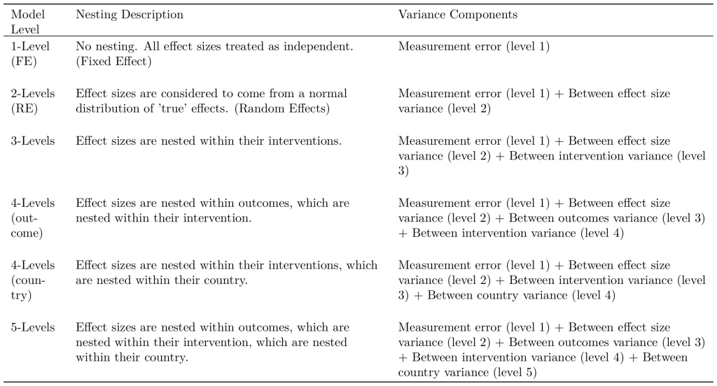
As aforementioned, our model has to at least be a random effects model. Multilevel models are expansions upon a random effects modelThe typical random effects model is actually a multilevel model with two levels to account for variation within effect sizes (due to sampling error, level 1) as well as variation between effect sizes (due to heterogeneity, level 2). Similarly, a fixed effects model only has one level that accounts for sampling error within effect sizes. . If we were selecting a model based only on theory we could select the 5-level model. However, we also consider model comparison (see Table C2).
Table C2: Model comparison.
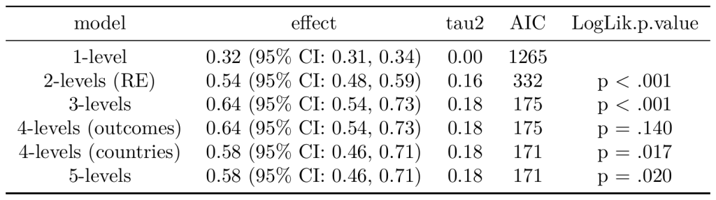
Note. τ2 are summed across all the levels for column ‘tau2’. The loglik p value is in comparison to the previous level (Level 2 vs Level 1, etc.), except for the 4- and 5- level models, which were all compared to the 3-level model.
We employed two widely used statistical criteria: the Akaike Information Criterion (AIC) and the Log-likelihood Ratio Test. AIC values (the lower the better) provide a measure of the model's goodness of fit while penalising for complexity, thereby helping to avoid overfitting. The Log-likelihood Ratio Test directly contrasts the likelihoods of nested models, offering insights into whether additional parameters significantly improve the model's fit to the data. The 5-level model did best in terms of model comparison. It is more conservative than the simpler 3-level model and includes the structure better than a 1- or 2-level model.
Note that the confidence interval more or less increases as we add more nesting; this is expected of RE and MLM models, as more heterogeneity means more uncertainty. However, the increase in the effect size is not always an expected pattern (although this also occurs in Tong et al., 2023, when they use a 3-level model). This increase may result from the reweighting process, where accounting for heterogeneity adjusts for dependence between effect sizes and shifts the results. But it could also be due to ‘small study effects’, either genuine or due to publication bias (Poole & Greenland, 1999; Borenstein et al., 2010). This does not mean we should use a different modelling specification, but that we should include publication bias adjustments. We address this more in Appendix E.
C4. Meta-regressions and moderator analysis
We are not just interested in estimating the average effect of psychotherapy. Instead, we want to explain why results from studies differ. To do this, we use a meta-regression. Meta-regressions are like regressions, except the data points (i.e., dependent variables) are effect sizes weighted according to their precision and the explanatory variables are study characteristics. Meta-regressions allow us to explore why effects might differ between studies. We consider how much the effect changes for the following characteristics: follow-up time (in years after the end of the intervention), dosage (as the number of sessions), delivery format (group or individual), expertise of the deliverer, control group type, population, and measure type.
Appendix D: Detail about main model
In this appendix we discuss in detail the main model from our meta-analysis.
We find that, on average, psychotherapy in LMICs has an effect of 0.58 SDs on the wellbeing of the recipients. This is much lower than if we had included outliers or high risk of bias studies (see Table D1 for more detail).
Table D1: Simple meta-analysis models.
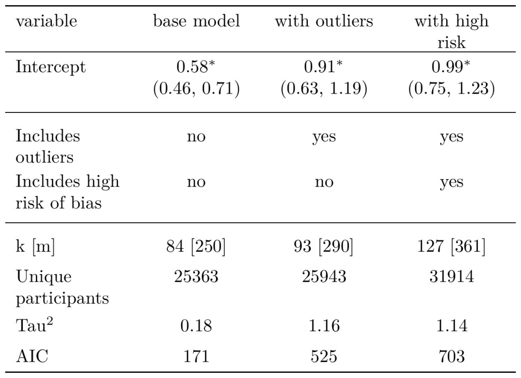
Note. All the effects presented above the first separation line are coefficients from the meta-analysis model. Their effects are in Hedge’s g (SD changes). The parentheses represent 95% confidence intervals. Statistical significance is represented such that * p < 0.05; ** p < 0.01; *** p < 0.001.
D1. Total effect over time
However, what we care about is the total effect over time on the recipient. To estimate the total effects of psychotherapy for its direct recipient we need to estimate the initial effect of psychotherapy and how long these effects last. To do so, we moderate the effect with the time in years since the end of the intervention. Hence the main model that matters to us is a meta-regression where we moderate the effect by time. This will provide us with an intercept that predicts the effect immediately after treatment has ended (the initial effect) and a coefficient that predicts the change in effect per year (see Table D2).
Table D2: Adding moderation over time.
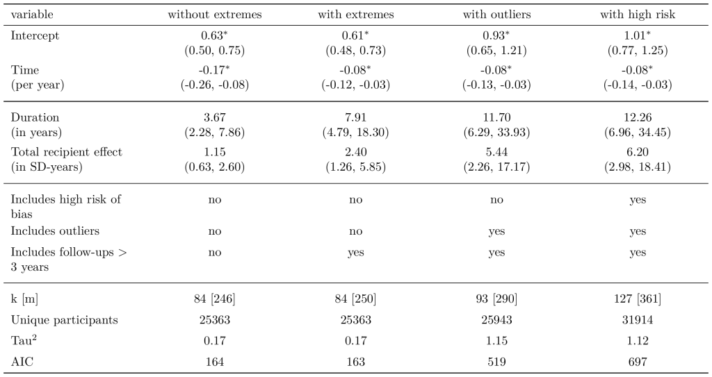
Note. All the effects presented above the first separation line are coefficients from the meta-analysis model. Their effects are in Hedge’s g (SD changes). The parentheses represent 95% confidence intervals. Statistical significance is represented such that * p < 0.05; ** p < 0.01; *** p < 0.001.
Taking these two parameters together, we can calculate the total recipient effect (i.e., the integral of the benefits over time for the recipient). Because we find a negative trajectory over time (a decay; the effects become smaller) and we model this as linear, this can be easily calculated using the formula for the area of a triangle (see Figure D1)For more detail this is calculated as an integral. To determine the uncertainty around the total effect we use Monte Carlo simulations (see our methods website page), calculating for each pair of simulations the integral. In order to avoid technical issues in our simulations, we prevent simulations of initial effects from being negative and we prevent simulations of decay from being positive. :
intercept * abs(intercept/decay) * 0.5
Figure D1: Different trajectories and integrals over time.
Note. The blue line represents the average trajectory over time (from post-intervention to when it reaches zero) according to the model without the extreme follow-ups and the red line represents that of the model with the extreme follow-ups. The respective shaded areas represent the integrated effect over time, the total recipient effect.
However, there are 4 effect sizes with follow-ups of 3 years or more from the Healthy Activities Program (4.87 years) and the Thinking Healthy Programme Peer-Delivered (THPP) in India (3.21 years) both reported on in Bhat et al. (2022). The next longest follow-up times are less than 1.5 years. These effect sizes could affect the modelling of the trajectory over time; therefore, we compare models with and without these. We can see that the extreme follow-ups exert a lot of influence on the model because removing them adjusts the total effect by a factor of 1.15/2.40 = 0.48 (a 52% reduction). In the case where the extreme long-term follow-ups are included, the effects are estimated to last 8 years before they reach an effect of zero, but when they are excluded this drops to 3.7 years. Note how much larger, and heterogeneous, the results would be if we had kept outliers and high risk of bias studies.
The effect sizes from the interventions of the extreme follow-ups are presented in Table D3.
Table D3: Characteristics of studies with long term follow-ups
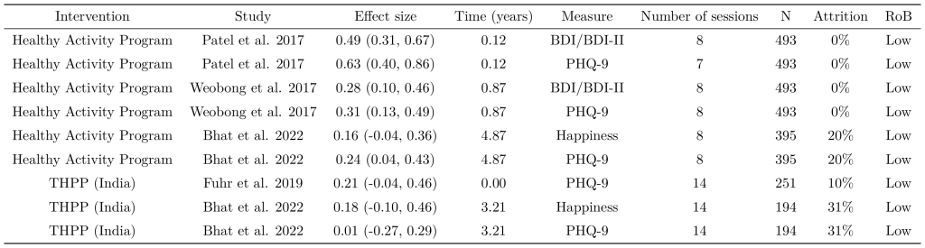
These effect sizes are ‘extreme’ with respect to their decay rates (when they are included, the decay becomes about 2 times weaker) and follow-up times (the next longest follow-up time for a study is ~1 year). This itself might not be a sufficient concern to exclude these. We want information about the duration of psychotherapy’s effects, and the studies that are most informative about how effects last are the ones with the longest follow-ups. However, these do exhibit a high degree of influence on our results. We are generally concerned about any small number of effects having a disproportionate effect on our results. We consider different reasons for whether we should be wary of these effects.
Are these results surprising? To some extent, yes. Bhat et al. (2022) collected 234 forecasts collected before the follow-up results were published. The forecasters expected the follow-up effects to be much lower than the reported results. The median prediction was 0.08 SDs, compared to a reported pooled effect of 0.23 SDs – the actual result only corresponded to the 10th percentile of highest predictions. In other words, these results were surprising. And there’s been some work to suggest that surprising results are, in general, less likely to replicate (Open Sci. Collab., 2015; Wilson & Wixted, 2018; Dreber et al., 2015).
Were these follow-ups planned only because the earlier results of the trials they are based on were unusually promising? This seems unlikely. The earliest effect sizes of these trials are not higher than the average effect of 0.58 SDs we found in our meta-analysis. Furthermore, we find that studies with more follow-ups in our meta-analysis, if anything, non-significantly predict lower initial effects.
Were these interventions much more likely to have long-term effects (higher dosage, greater expertise, etc.) than others? This seems unlikely. The characteristics of these studies appear largely unexceptional. All of these programmes were delivered by non-experts, which, as we show in Appendix G, is related to a smaller effect. While the THPP has an above-average number of sessions (14 compared to the average 7.18 in the model without extreme follow-ups), the number of sessions does not significantly predict the effect or the persistence of an effect (see the dosage and time interaction model in Appendix G). However, in a weighted regression, we find a significant relationship between the number of sessions and the length of the latest follow-ups of interventions.
A further issue is attrition. The attrition in these studies is higher (20 to 30%) than for the average follow-up for studies at six months (8%)These figures come from comparing the baseline to follow-up sample size. However, this underestimates attrition because when studies were using ITT we had to extract the full sample size used for the ITT results in order to have the right calculation for the effect size. It would take more time to extract detailed attrition figures. and higher than other development RCTs (k = 14) with long-term follow-ups between 7 and 10 years (5-14%; Bouguen et al., 2018). However, Bhat et al. argued that the attrition in their respective studies is similar between treatment and control conditions. While this is somewhat reassuring, we cannot rule out that attrition is due to unobservable confounders related to the treatment condition or control conditions (e.g., it just so happens that participants dropped out across groups in equal proportions due to poor mental health in the treatment group, and good mental health in the control group – the worst, but admittedly imaginative, case).
On the other hand, studies should be excluded only when we think they present truly anomalous results. However, these effect sizes are from studies which appear to be of a relatively higher quality than most studies in our meta-analyses. They are well powered and Bhat et al. was pre-registered – signs that a study is likely to reproduce (Nosek et al., 2022). These interventions were rated as ‘low’ risk of bias. Plus, the results also behave in a reassuringly intuitive manner: within these studies’ follow-ups, the effects decline dramatically.
The important role that psychoeducation could play in LMICs, where there is less awareness than in HICs (see Appendix H), could explain why longterm benefits could occur. We also think the duration estimate of our model is plausible given the broader evidence around the long term effects of psychotherapy on criminal behaviour at 10 years (Blattman et al. 2022); or depression in HICs at 3-5 years (Wiles et al. 2016), 5-8 years (Tyrer et al. 2017; Tyrer et al. 2020), 5 years (Kohtala et al. 2017; Mulder et al. 2022). Baranov et al. (2020) found a significant effect of psychotherapy at 7 years in Pakistan, albeit on a semi-structured clinician interview which does not fit our inclusion criteria.
Overall, we should be very cautious about having our results being driven by these 4 effect sizes, but to dismiss this evidence entirely seems unjustified. These studies should still update our views towards the durability of psychotherapy’s effects, even if we do not rely on them entirely. Unfortunately, we have not found a clear academic precedent to help us decide which specification we should use. We welcome more expert feedback in this domain. In light of that, instead of taking the long-term follow-ups at face value or completely excluding them (the conservative case), we take a middle road approach where we weight each model. Unsure how best to combine these models, we apply a naive 50-50% averageAs a sanity check, we can see how much a Bayesian process would update if we consider the decay rate without the long-term follow-ups, -0.17 (95% CI: -0.27, -0.07) as a prior and the estimated decay rate with the long-term follow-ups, -0.07 (95% CI: -0.11, -0.03) as the new evidence. In that case, using Bayes’s rule with a normal-normal conjugate suggests a posterior decay rate of -0.09 (95% CI: -0.13, -0.05), updating closer to the evidence with the extreme follow-ups (this is because their inclusion considerably shrinks the standard error of the estimated decay rate). This is somewhat reassuring that our more moderate update based on the long-term follow-ups is not unreasonable. However, we are still double counting the information from the rest of the meta-analysis. to the total effects of the model with and the model without the extreme follow-ups. This results in a total effect of 1.15 * 0.5 + 2.40 * 0.5 = 1.78 SD-years. Because we still need a model to be used for the other moderations, publication bias, and as priors for our charity cost-effectiveness analyses, we take the conservative model (which removes the extreme long-term follow-ups) but apply an adjustment factor of 1.78/1.15 = 1.54 to its total effect. One issue here is that we are double counting the information from the rest of the meta-analysis (most effect sizes are in both models).
We recognize that this is an important value in our analysis, and think reasonable people could disagree about the right approach and/or weighting. We present the influence of this decision point in our robustness checks (see Appendix O2).
D2. Removing bias from Iranian studies
A disproportionate amount of psychotherapy RCTs were conducted in Iran (recall that our inclusion criteria is not just studies in SSA but in LMICs more generally). Even after removing outliers and ‘high’ risk of bias studies, there was a high proportion of effect sizes from Iran (see Table D4).
Table D4: Distribution of interventions and effects across countries.
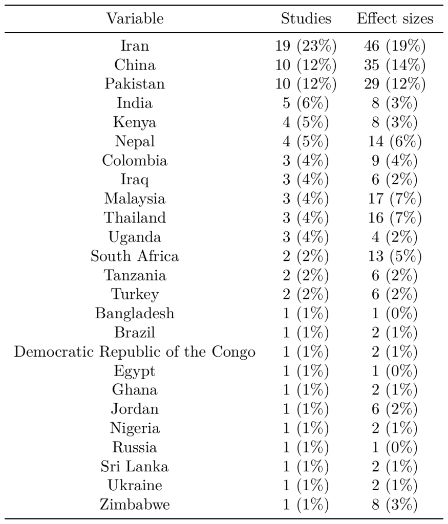
We are not sure why this is, but during our first extraction we had internally noted that many of these RCTs appeared to be of questionable quality for reasons outside of those captured by RoB (e.g., underpowered sample sizes, typos, poor formatting, inconsistent reporting of figures). Furthermore, Iran has been identified as one of the countries with issues of fake academic papers (Else & Van Noorden, 2021; Richardson et al., 2024). We are not saying these are fake studies, just that this is an additional reason for our scepticism.
We did some exploratory modelling and found that adding an indicator for whether study was based in Iran added a lot of explanatory power to our model. This indicator significantly predicts that studies from Iran have much higher effects than studies in other countries by 0.38 SDs. For instance the Iran model implies that the average initial effect in other countries is 0.59 SDs but 0.59 + 0.38 = 0.97 SDs in Iran.
In terms of causal modelling, we consider Iran to be a confounder, where characteristics of Iranian studies might affect results directly rather than only through changes in treatment. We interpret this as bias, since we do not think there are credible reasons for interventions in Iran to be exceptionally effective. A further reason for treating this as bias is that we do not find this pattern if we use China – the next highest providers of effect sizes in our analysis – as a predictor (instead, the effect is small and non-significant). Similarly, there is no significant effect from world regions (compared to Sub-Saharan Africa, where the charities operate), other than for the Middle East, which is no longer significant once we control for Iranian studies.
Note that bias from Iran does not significantly interact with trajectory over time (plus, at face value, it would suggest that Iranian studies had more decay). Hence, we only adjust the intercept. See Table D5 for a summary. Because of this, we decided to add Iran as a predictor in our core modelWe do not simply exclude Iranian studies because we do not think we have sufficient ground to do so. It is not in our protocol and these studies were not removed through removal of outliers or ‘high’ risk of bias studies., which reduces the initial effect of psychotherapy and therefore its total effect (see Table D6).
Table D5: Effect of study region.
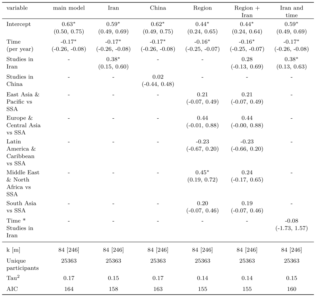
Note. All the effects presented above the first separation line are coefficients from the meta-analysis model. Their effects are in Hedge’s g (SD changes). The parentheses represent 95% confidence intervals. Statistical significance is represented such that * p < 0.05; ** p < 0.01; *** p < 0.001
Table D6: Primary moderators for general evidence of psychotherapy.
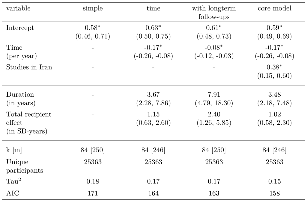
Note. All the effects presented above the first separation line are coefficients from the meta-analysis model. Their effects are in Hedge’s g (SD changes). The parentheses represent 95% confidence intervals. Statistical significance is represented such that * p < 0.05; ** p < 0.01; *** p < 0.001
Appendix E: Publication bias
E1. What is publication bias
Publication bias is “when the probability of a study getting published is affected by its results” (Harrer et al., 2021). Publication bias is widespread in social science generally (Franco et al., 2014). When it is identified, it should be corrected for. There are three different types of bias worth distinguishing because they are assessed and adjusted for in different ways.
Small studies effects: Studies with small sample sizes – which consequently have large standard errors (SE)The standard error quantifies how much an effect size varies from the ‘true’ population effect. The smaller the standard error, the more accurate the effect size. Studies with small sample sizes have larger standard errors because small samples are less representative of the entire population. This is related to the law of large numbers. – are assumed to be more likely to fall prey to publication bias because only small studies with large effect sizes will be published. Note that there can be small studies effects due to genuine patterns other than publication bias (e.g., the treatment works best for a specific population that is smaller, and so can only be studied with small samples; Sterne et al., 2001, 2004).
Selection based on significance: Publication is not only influenced by the magnitude of the effect size, but also by its significance. That is, findings are typically considered worth publishing when p < .05. Here we look for certain patterns of evidence involving p-values that might suggest practices like p-hacking.
Time-lag bias (or winner’s curse) is where earlier studies tend to have larger effect sizes than the later ones. This can happen because new findings about a phenomenon will more likely be published if they are larger and/or significant. Over time, as more research accumulates, the reported effect sizes tend to decrease and converge towards the actual effect, which may be more modest
E2. Diagnostics
The first step is to diagnose whether there are signs of publication bias in our data.
E2.1 Small studies effects
For bias based on small studies effects, detection tools look at whether there is a certain pattern relating the size of effects and their SE. We use the typical methods for detection here (Harrer et al., 2021).
One tool is the funnel plot (Peters et al., 2006, 2008; see Figure E1), which allows for a visual inspection. The effects are plotted against their standard error. A funnel plot also includes a line for the pooled effect of our meta-analysis. This allows us to see how effect sizes are distributed around the effect (which ones are lower or higher). It also plots a cone for the expected (or pseudo) confidence interval in which we expect to see the studies around the pooled effectThis is neither the confidence interval or the prediction interval of the model, rather, it is a simple calculation of a confidence interval for each level of SE plotted (pooled effect ± z * SE). We also added a contour plot, which is an interval around 0 that indicates to us whether the effect sizes are significant or not (i.e., it allows us to also observe some selection based on significance; Peters et al., 2008). This is neither the confidence interval or the prediction interval of the model, rather, it is a simple calculation of a confidence interval for each level of SE plotted (0 ± z * SE). . If there are some studies on one side (notably the right hand side because those are studies with higher effects) but not on the opposite side, this suggests some asymmetry which can indicate publication bias. The plot is complicated but we can see a few patterns: there is a lot of spread, a lot of the more precise effect sizes have lower effects (and less likely to be significant) than the average (top left), and there are a few less precise effect sizes on the right hand side without equivalents on the left hand side. Overall, this does suggest that small studies effects are occurring.
Figure E1: Funnel plot.
Note. The dotted lines represent the funnel. The shaded grey contours represent the contour plot. The points represent the different effect sizes.
But a funnel plot is not a quantitative method. Instead of relying on visual inspection of the relationship between SE and effect sizes, we can test it with Egger’s regression (Sterne & Egger, 2005). In this test, effect sizes, standardised by their respective SE (i.e., a z-score), are regressed against the precision (i.e., the inverse of the SE). The intercept from this regression model represents the effect size when the precision is zero (i.e., when the SE is infinitely large). An intercept of zero would indicate that there is no small studies effects, as it would mean that the SEs and the effect sizes are unrelated. Conversely, a non-zero intercept, especially if statistically significant, would suggest the presence of small studies effects (see Harrer et al., 2021, for more detail). In our case, the intercept is significantly different from zero (b0 = 2.49, p < .001), which implies that there is asymmetry and relationship between SE and effect sizes (see Figure E2).
Figure E2: Egger’s regression.
Note. The full line represents Egger’s regression, the dashed line represents an intercept of 0, and the dotted line represents where the regression line should be if it didn’t have a shifted intercept.
More intuitively, a PET model is a meta-regression model where we moderate the effect sizes with their SE. According to this model, higher SEs will significantly lead to higher effect sizes (b1 = 2.04, p < .001).
Note that none of these methods fully account for the structure of our model, where we use a multilevel model with a time and an Iran bias moderator (these methods are made for fixed effect or random effects models without moderators). For example, the funnel plot cannot differentiate between small effects that are due to longer follow-up times from generally smaller effects. Nakagawa et al. (2021) proposes a model that builds on the PET model which can account for moderators and multilevel structures. It also suggests that higher SEs will significantly lead to higher effect sizes (b3 = 1.59, p = .001).
E2.2 Selection based on significance
Here we consider methods that investigate whether publication bias might be due to selection of presented results based on p-values. This can be due to authors only publishing statistically significant results or due to p-hacking (tweaking the analysis and running multiple models but only reporting those with significant results).
A common method to detect result selection is the p-curve (Simonsohn et al., 2014a, 2014b, 2015). This model analyses a distribution of all the p-values below 0.05 of the dataset. Under the null hypothesis (i.e., if there is no effect), the distribution of p-values should be uniform (flat). If there is a true effect, the distribution will be right skewed (more highly significant and smaller p-values will be found more often). p-hacking is indicated by a left-skew, because researchers would be including more p-values close to the significance threshold (.05) than there should be. An uptick around the p-value of .05 would also be suspicious. The uptick around the p-value of 0.5 is ever so slight. The skew is very much to the right; plus, the significant tests for right-skewness suggest that we are indeed detecting a true effect of psychotherapy (see Figure E3). This does not present a strong case of publication bias.
Figure E3: p-curve.
We also use the z-curve (see Figure E4), which is a rather novel method that expands on some of the principles of p-curve (Schimmack, 2021; Bartoš & Schimmack, 2022). The z-curve is a distribution of the z-values of the studies in the dataset (z-values are the number of standard deviations a number is away from the mean. Here, we calculated them from the p-values). The p-curve bins all the .01 values (z > 2.58; the black line) together, but the z-curve shows their distribution. This allows us to see if there are more subtle p-hacking patterns; notably, if a lot of the data is actually close to the .05 threshold (red line). There seems to be more results around that threshold. Moreover, the observed discovery rate (the percent of significant p-values in the dataset) is higher (although still within its CI) than the expected discovery rate (the expected percent of significant p-values produced by a dataset with this distribution of power), which is tentative evidence that some selection bias is occurring. The curve in the z-curve extrapolates the distribution according to the expected power of the data, showing that more non-significant studies (z < 1.96) are expected, providing further evidence of selection bias.
Figure E4: z-curve.
E3. Correction methods
The diagnostic tools suggest there is publication bias in our data. Therefore, we investigated different publication bias correction methods. We selected different popular methods based on simulation studies and guidelines (Carter et al., 2019; Hong & Reed, 2020; Harrer et al., 2021): trim and fill, PET-PEESE, Rücker’s limit meta-analysis, UWLS-WAAP, 3PSM, p-curve, and RoBMA. We do not include a simple fixed effect model among these for reasons described in this footnoteSome studies (Stanley & Doucouliagos, 2015, 2017) have shown that, in cases of small studies effects, fixed effect (FE) models can be less biased than random effects (RE) models – the type of model we use (our MLM model is building upon a RE model; see Appendix C). However, this does not mean that it is appropriate to use a FE model because, as discussed in Appendix C, the choice of FE or RE models is about the structure of the population of effects. The population effects are clearly not homogenous. As we explored in our moderation analyses, differences in psychotherapy characteristics clearly relate to its effectiveness. Instead, when there is publication bias, this means we need to add a correction method to our estimate, as we do in this analysis. We confirmed this by contacting three experts from the meta-analysis literature. Harrer and Borenstein both confirmed that this was the appropriate method and that we should use our current model with publication bias correction and sensitivity analyses. Stanley suggested we should use two publication bias correction methods he is an author for: UWLS-WAAP and RoBMA, which we include in our adjustments for publication bias. Furthermore, in our own unpublished simulation analysis based on the data from Carter et al. (2019), we found that ‘RE + a correction method’ tended to outperform ‘FE + a correction method’ for contexts like that of our meta-analysis.. Our model of interest is one with a moderation over time (and for bias from Iran) so we can calculate the total effect. Furthermore, our model involves a multilevel structure. None of the typical publication bias correction methods can be applied to such models. Therefore, we also use a new method by Nakagawa et al. (2021, correction; which we name ‘the Nakagawa method’) which builds upon PET-PEESE by introducing multilevel structure, moderator variables, and a test for time-lag bias.
Trim and fillWith a L0 fixed-random algorithm (Peters et al., 2007). reduced the effect by filing 91 effects. This is a popular and long-established publication bias correction method (Duval & Tweedie, 2000b) that uses an algorithm to iteratively remove effect sizes until there is no longer asymmetry in the funnel plot, then reinstating these effect sizes with mirrors of the effect sizes to compensate for the asymmetry they produce. This method is usually found to be flawed in simulation studies (Carter et al., 2019) and its error increases with heterogeneity (Peters et al. 2007; Terrin et al. 2003; Simonsohn et al., 2014b; Weinhandl & Duval, 2012). Hence, because of the high heterogeneity in our data, it will not perform well.
A typical method that is more modern than trim and fill is PET-PEESE (Stanley, 2008; Stanley & Doucouliagos, 2014; Stanley, 2017; Harrer et al., 2021). It is a continuation of the logic of Egger’s regression. It moderates the effect sizes with their SE, thereby telling us whether the SE significantly predicts the overall effect, and predicts what the effect would be if the influence of SE was set to zero (i.e., the limit effect). PET uses the SE, whereas PEESE uses the variance. PET-PEESE accounts for the fact that PET has a downward bias if a true effect is detected by selecting PEESE when a true effect is detectedIf the intercept of the PET model is greater than 0 and significant at the 0.10 level.. Our implementation of PET-PEESEWe use a meta-analysis version (additive error) with a RE model which is also how the large simulation studies implemented it in their code (Carter et al., 2019; Hong & Reed, 2020). We use corrected SEs (Pustejovsky & Rogers, 2018; Harrer et al., 2021) that recalculate the SEs without using the effect size in them, thereby, removing some in-built correlation between the effect size and the SE. confirms that there is a relationship between the SE of the effect sizes and the effect sizes themselves, and selects a PEESE correction accordingly.
Another method that uses the principles of limits and relation with the SE is Rücker’s limit meta-analysis (Rücker et al., 2011; Harrer et al., 2021). This directly incorporates the τ2 in the calculation of the adjusted meta-analysis and can also adjust the individual effect sizes themselves.
Unrestricted weighted least squares - weighted average of the adequately powered (UWLS-WAAP) is a method developed by Stanley and colleagues (Stanley & Doucouliagos, 2015; Stanley et al., 2017). The UWLS part is a modelling that is different from both FE and RE. It will have the point estimate of an FE, but includes heterogeneity in the calculation of the confidence interval (i.e., wider CIs than for FE). It is calculated using a linear regression (a multiplicative model of errorOur current modelling assumes an additive model of error (SE and τ2are added together but not correlated). Stanley et al. (2022) suggest that if SE and τ2are correlated, then a UWLS model would be more appropriate. The VR-MRA test (Stanley et al., 2022) suggests that the SE significantly increases with heterogeneity in our data. However, we do not use UWLS as our primary model specification because (1) it does not deal with the dependencies between our effect sizes (i.e., it is not a multilevel meta-regression) and (2) the publication bias adjustment it suggests is severe but in line with other models and incorporated in this analysis when we combine the models (see Appendix E4).). WAAP is the final step of the model. It reruns the UWLS, having filtered out any study that is not powered enough to detect the pooled effect size of the UWLS, providing a new estimate of the pooled effect.
The p-curve can also adjust for publication bias by finding the pooled effect size that best fits the distribution of p-values (Simonsohn et al., 2014b). However, van Aert et al. (2016) showed some limitations of the p-curve, notably that when heterogeneity is high (I2 > 50%) – which is the case in our data – the p-curve adjusted estimate of the effect size shouldn’t be trusted because the p-curve method tends to overestimate the effect size.
An alternative method to correct for publication bias due to selection of significant effects are selection models. We use a common step function selection model called three-parameter selection model (3PSM; Vevea & Hedges, 1995; Vevea & Woods, 2005). This model’s theory is that p-values between 0.025 and 1 are differently weighted compared to p-values below 0.025. We find significant evidence that effect size with p-values between 0.025 and 1 are less likely to be selected than those below 0.025. This is evidence in favour of publication bias, so the model adjusts the pooled effect size for it.
The RoBMA method (Bartoš et al., 2022) does Bayesian averaging (the most informative posterior informs the overall average the most) of different methods (PET-PEESE and multiple selection models). Proponents of the RoBMA method might argue that this is the way to incorporate different methods (see Section E4 for more discussion). However, this method does not incorporate the Nagakawa method (see below) nor the limit meta-analysis. It does not deal with moderators nor with the multilevel structure that is of interest to us. Instead, we add it to the different methods that we combine together.
Our model of interest is a multilevel model with a moderation over time (and Iranian bias) so we can calculate the total effect. Furthermore, our model involves a multilevel structure. None of the typical publication bias correction methods can be applied to such models. The Nakagawa method (2021, correction) can deal with this. Hence, we can reproduce our model of interest with the moderating effect of time by adding the effect of the SE. It also confirms that there is an effect of the SE on the effect sizes, and selects a PEESE-equivalent correction (i.e., using variance).
With the Nakagawa method we can also test the effect of year of publication (time lag bias). We find a significant effect of time-lag bias: each further year of publication reduces the effect by -0.02 SDs; hence, newer studies have smaller effect sizes. However, we do not include this in the Nagawaka method we use for determining the publication bias adjustment because it has a higher (i.e., less corrected) total effect integrated over time with the year of publication moderator (0.81 SD-years) than without (0.72 SD-years); namely, it leads to more lenient publication bias adjustment, so we select the harsher more conservative one for this method.
E4. Combining the correction methods
There are three ways of dealing with publication bias (Carter et al., 2019; Harrer et al., 2021; Bartoš et al., 2022): (1) Pick one correction method and apply it. (2) Apply different correction methods and present how sensitive the results are to each of these. (3) Average across different methods. No method of publication bias adjustment systematically out-performsPerformance is determined by measures of error or distance from the intended ‘true’ effect which is known in simulation studies because authors set the characteristics of the data that is simulated. the others (Carter et al., 2019; Hong & Reed, 2020); hence, it seems inappropriate to only pick one method. The Nakagawa method is the most appropriate for our modelling purposes but we do not think its greater compatibility with our modelling approach is sufficient grounds for us only using this method. It is still a new and relatively untested method. Instead, we prefer to combine information from all the methods.
We combine information from each method by calculating how much it reduces the effect. The Nakagawa method provides us with an estimate of the initial effect and the decay, so we can calculate the total recipient effect and compare how much of a reduction it is to our core model (see Section 4.1). The other methods cannot account for moderation over time nor the multilevel structure. Hence, we compare their reduction in the intercept to the intercept of their own reference point; namely, an intercept-only RE model. We then apply that proportional reduction to the total effect of the main model. The models and relative changes are presented in Table E1, at the end of this section. This also allows readers to see how sensitive results would be to different methods. adjustments ranging between 0.38 and 0.99, except for the p-curve that suggests an increase (by a factor of 1.10). A range of results is to be expected from different models (Carter et al., 2019; Hong & Reed, 2020), as they operate in different ways. The naive average of these is 0.69 (a 31% discount)If we remove the two worst performing methods according to simulation studies, the Trim and Fill and p-curve methods, the adjustment remains very similar at 0.66 (a 34% discount).. We discuss sensitivity of publication bias to the exclusion of outliers and high risk of bias studies in Appendix P.
Table E1: Publication bias correction methods.
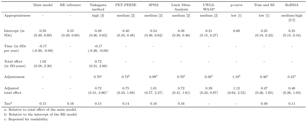
Note. The parentheses represent 95% confidence intervals.
Appendix F: Range restriction
We use Cohen’s d and Hedges’s g, a common form of standardised mean difference (SMD), to standardise effect sizes in our meta-analyses. Using SD changes is the dominant way meta-analyses standardise effect sizes for continuous outcomes (Higgins et al., 2023; Harrer et al., 2021). We have to do so because we are combining results from different studies with different measures of subjective wellbeing (SWB) and affective mental health (MHa) with different scale lengths. This involves dividing the raw treatment effect (the difference between the control and treatment group outcomes) of an intervention by the pooled standard deviation of the sample (i.e., the pooled variance; a weighted average of standard deviations or variance between control and treatment groups). The resulting standardised effect size is interpreted as SD changes. However, this means it is technically possible to increase the effect size either by increasing the treatment effect (what we assume most people care about) or decreasing the variance of the outcome (we exemplify this in Appendix F2.1 with other notes on range restriction).
In practice, this is a particular concern with psychotherapy trials, which commonly only include participants who are mentally unwell. Namely, it selects participants based on a cut-off on the outcome of interest, the affective mental health (MHa) measure. This restricts the variance of mental health scores we observe compared to the alternative where a general population is treated. This is not an issue with other interventions such as cash transfers, where recipients are selected based on other criteria, like poverty, which is not a direct measure of subjective wellbeing or affective mental health.
This artificial shrinkage in the variance of mental health scores very plausibly leads to an overestimate of psychotherapy’s standardised effect sizes. This phenomenon is referred to as ‘range restriction’ or ‘range enhancement’ (Hunter & Schmidt, 2004; Wiernik & Dahlke, 2020; Harrer et al., 2021) and can be corrected if one knows the variance in the target population. However, this is not the case for us because we have many different studies, with different measures, across different countries. Instead, we apply a general adjustment calculated from general trends in the restriction of variance for mentally distressed populations that we explore in large datasets.
F1. Using large datasets to estimate psychotherapy’s range restriction
We explore whether SMD overestimate effects on MHa because psychotherapy selects recipients based on the outcomes. We use multiple datasets with a general population of respondents who have answered a depression scale. This allows us to split the sample based on common depression thresholds (i.e., the scores at which respondents are considered to have depression) to see if the variance on that scale becomes smaller for depressed respondents than for the whole sample (general population; i.e., including both depressed and non-depressed).
We use the thresholds for depression or distress (also called cut-offs) that a study mentions. Otherwise, we use the threshold that appears to be the convention in the literature. Note that different studies will suggest different cutoffs (Cornelius et al., 2013; Stolk et al., 2014). The data we use is summarised in Table F1 below.
We used three panel datasets (BHPS, n = 219,619, UK; HILDA, n = 84,695, Australia; NIDS, n = 96,412, South Africa) and two datasets from RCTs in LMICs (Haushofer & Shapiro, 2016, a cash transfer study, n = 1,569; Barker et al., 2022, a psychotherapy study included in our analysis, n = 6,205) to estimate the size of this bias. We found that, when only selecting the participants who pass a threshold for depression, the SD of MHa scores is between 69% and 99% of the SD of MHa scores when including the whole population (including all participants, both those who pass and do not pass the threshold). We take an averageBecause these are all on different scales, we cannot average the variances themselves and instead average the percentage change. (weighting on the number of depressed respondents) of the change in the variance between the general population and the variance of the subgroup that passes a threshold for mental distress. On average, the variance for individuals past the threshold for mental distress becomes 0.88 (12% smaller) of that of the general population’s variance. Because the variance is on the denominator, this inflates effect sizes by 1 / 0.88 = 1.14. Which means that we need to apply an adjustment factor of 0.88 (a 12% discount) to correct for this.
However, this discount will only apply to the effect sizes where participants were selected based on a mental health cut-off (either on the outcome scale or a clinician diagnostic) and where responses are given on affective mental health measures (see below about subjective wellbeing measures). This is the case for all of the charity-related causal and pre-post data. However, this only represents 64% of effect sizes in our general meta-analysisThis represents 65% of the weight of the meta-analysis but we use the percentage of studies because it is close and easier to to understand.. Adding this correction suggests that, to adjust for psychotherapy inflating SMDs, the adjustment factor would be 1 * 0.88 * 0.64 + 1*(1-0.64) = 0.92 (a 8% discount).
We also tested, using the same datasets, whether restricting samples on mental health status shrinks the variance of life-satisfaction, to see if this issue generalises to SWB measures, but we found it does not (see Appendix F2.2).
Table F1: Sources of evidence for sample restriction effects on SWB and MHa scores
|
source |
country |
country type |
waves |
n general |
n depressed |
MHa measure |
Cut- off |
SD for MHa (general) |
SD for MHa (depressed) |
Change in SD for MHa |
LS measure |
SD for LS (general) |
SD for LS (depressed) |
Change in SD for LS |
|
BHPS |
UK |
HIC |
18 out of 18 |
219,619 |
85,463 |
GHQ-12 (0-36)General Health Questionnaire (GHQ-12; Golberg et al., 1997). 12 items with scores ranging from 0 to 36. We use the threshold of 12, because this is the recommended threshold for the likert coding version of this questionnaire (which is used in the BHPS). |
12 |
5.43 |
4.90 |
90% |
life satisfaction (1-7) |
1.77 |
1.84 |
104% |
|
HILDA |
Australian |
HIC |
6 out of 17 |
84,695 |
31,610 |
K10 (10-50)Kessler Psychological Distress Scale (K10; Kessler et al., 2002). 10 items with scores ranging from 10 to 50. There is a lot of variability in how the cut-off is determined (Stolk et al., 2014). We use the K10 scores from the HILDA survey, and this dataset refers to Australian Bureau of Statistics’s guidelines; hence, we use their proposed cut-off of 16 for moderate psychological distress. Barker et al. (2022) also use K10, but they use a cut-off of 20. |
16 |
6.53 |
6.47 |
99% |
life satisfaction (0-10) |
1.43 |
1.65 |
115% |
|
NIDS |
South Africa |
LMIC |
5 out of 5 |
96,412 |
24,352 |
CESD10 (0-30)There is a 10 item version (CESD10) with scores ranging from 0 to 30 for which the recommended cut-off is usually 10 (Andresen et al., 1994). |
10 |
4.40 |
3.03 |
69% |
life satisfaction (1-10) |
2.44 |
2.35 |
96% |
|
Haushofer & Shapiro, 2016 |
Kenya |
LMIC |
single study |
1,569 |
1,336 |
CESD20 (0-60)There is a 20 item version (CESD20) with scores ranging from 0 to 60 for which the recommended cut-off is usually 16 (Weissman et al., 1977) but some more recent meta-analytic work suggests a cut-off of 20 might be more appropriate (Vilagut et al., 2016). However, because the cut-off of 16 is also what Hausehofer et al. (2020) used in their analysis, we use 16. |
16 |
9.92 |
8.30 |
84% |
life satisfaction (z-score) |
1.04 |
1.02 |
98% |
|
Barker et al., 2022 |
Ghana |
LMIC |
single study |
11,298 |
6,205 |
K10 (10-50) |
20 |
7.66 |
5.92 |
77% |
life satisfaction (z-score) |
1.00 |
0.98 |
98% |
Note. BHPS = The British Household Panel Survey, HILDA = The Household Income and Labour Dynamics Survey, NIDS = National Income Dynamics Study. MHa = affective mental health measure (e.g., depression). LS = life satisfaction.
F2. Other notes about range restriction
F2.1 Exemplifying the logic of changes in variance for SMDs
We try to illustrate the role of variance in SMD. Let’s imagine there is two interventions: A and B with the same raw effect but different pooled standard deviations – this would lead to a higher Cohen’s d for intervention A than intervention B. See Table F2.
Table F2: Example of Cohen’s d and the role of variance.
|
Intervention |
Control group mean (SD) |
Treatment group mean (SD) |
Raw effect on the same scale (e.g., 0 to 10) |
Pooled SD of outcome |
Cohen’s d |
|
A |
5 (3) |
6 (1) |
1 |
2 |
0.5 |
|
B |
5 (4) |
6 (4) |
1 |
4 |
0.25 |
Note. For simplicity of the example, we are assuming the groups have the same sample sizes and the pooled SD is calculated with (SD1 + SD2)/2 rather than the full formula.
Taking into account the SD of the groups (the variance) in quantifying the difference between groups is a part of Cohen’s d. Namely, it is comparing the two groups as two subpopulations normally distributed with a certain mean and SD. The narrower the pooled SD, the further away the two populations are. Put differently, if you randomly sampled someone from the control group and the treatment group, Cohen’s d represents of how far apart they would be from each other. Taking the example interventions in the table above and simulating each group, we find that two random samples find the treatment person having a higher score 64% of the time in Intervention A, and only 55% of the time in Intervention B. Hence, there is less overlap (more distance) between the groups in Intervention A than Intervention B. The values in Table F2 are represented in Figure F1.
Figure F1: Illustrating the logic of SMD.
However, this phenomenon is problematic if the variance of the outcomes are artificially reduced in a systematic manner in one intervention compared to others (i.e., ‘range restriction’). In practice, this is a particular concern with interventions that select people for treatment based on the outcome used to measure the effect. Psychotherapy trials commonly only include participants who pass a threshold of symptoms of a mental illness (e.g., distress or depression). This is not an issue with other interventions such as cash transfers, where recipients are selected based on other criteria like poverty, which is not a direct measure of subjective wellbeing and affective mental health. For this reason it seems likelier that for a given measure of mental health (or subjective wellbeing, but see below), the variance in outcomes will be smaller in psychotherapy trials than cash transfer trials. And this shrink in variance would lead to an overestimate of psychotherapy’s effects. Again, the same expectation of overestimation would hold for comparing the SMD of other interventions if they select on the outcome of interest.
F2.2 Does range restriction overestimate SWB effects?
Our analysis also includes more classical SWB measures such as life satisfaction (LS). Additionally, we expect LS and depression outcomes to be correlated, so a restriction on one would probably apply to the other. Hence, we also investigated whether there is a lower variance in life satisfaction when you screen for baseline depression using the same datasets (see Table F1).
We found that, when only selecting the participants who pass a threshold for depression, the variance of LS scores is between 96% and 115% of the variance of LS scores when including the whole population (including all participants, both those who pass and do not pass the threshold). Hence, the variance for LS does not become smaller because of selection on the MHa outcome. On average (weighting on the number of depressed respondents), the variance for individuals past the threshold becomes 105% of that of the general population’s variance (102% when not weighted). This does not suggest a change for LS variance.
This is surprising. As we clearly illustrated above, when you reduce the range of values an outcome can take, this should shrink its variance. It seems like this should also be the case when you look at the variance of an outcome when you restrict the range of a highly correlated variable. These results might suggest that life-satisfaction and MHa aren’t correlated enough for reduction of the variance in depression outcomes to clearly influence the variance of LS outcomes. Hence, we do not select an adjustment for range restriction for SWB outcomes.
F2.3 Other analysis using our meta-analytic data
We also explored in our meta-analysis whether studies who select participants based on a mental health cut-off have higher results than those who do not (we removed studies on the general population – i.e., not suffering from mental distress – to make the comparison more meaningful). Studies with cut-offs show a non-significant increase in effect by 0.11 SDs. This suggests that the effect of these studies could be (0.58+0.11)/0.58 = 1.19 times higher than for those who do not select based on a cut-off (rather than the 1.14 times calculated above). We do not use this evidence as we believe it is much weaker because it is based on across-study differences rather than within-study differences and thus subject to confounding by other study-level differences. Notably, part of this increase in effect could be explained by range restriction, but part of it could be explained by other factors, such as genuinely leading to better results because treating individuals with worse symptoms could be more impactful (see Appendix G).
Appendix G: Detail about moderators
In this appendix we discuss in detail the different moderators that we include or consider including in our analysis. This is important for our external validity adjustments (see Section 5.2) and for our general understanding of the literature. In Appendix G1 we discuss calculating the general moderation adjustment. In Appendix G2 we discuss modelling and calculating dosage. In Appendix G3 we discuss other moderators. In Appendix G4 we summarise different models.
G1. Calculating the moderator and dosage adjustments
As mentioned in Section 5.2, we have built our moderator model based on theory of what variables explain important characteristics of the charities: whether the delivery was from an expert or a lay person, whether the delivery was to groups or individuals,
Ideally, in this model, we would have added the following moderators: dosage, whether the studies used ‘extra controls’ (active controls or enhanced usual treatment, which is not what recipients would typically counterfactually have access to), and whether the population treated is mentally distressed or not. However, none of these variables are significant and they complicate the modelling. For simplicity (and also as a conservative choice because this would have softened the adjustmentsHaving extra controls (enhanced usual care and active control) and being a general population suggest lower effects. But the charities treat people who are distressed and do not have access to the kind of treatment involved in the extra controls. Therefore, these would be upwards adjustments because this is not selecting a negative effect.) we decided not to include them.
Friendship Bench delivers 1-1 psychotherapy, via lay-therapist, to individuals with mental health problems, who have no enhanced alternatives to psychotherapy. We adjust the general meta-analysis of psychotherapy as source of evidence for Friendship Bench by 0.90 (10% discount) for using lay therapistsThe adjusted intercept is calculated as 0.75 (intercept) + -0.17 * 0 (setting time to 0) + 0.27 * 0 (not Iran) + -0.07 * 0 (not group therapy) + -0.22 * 1 (lay therapist) = 0.53. Therefore, the adjustment is 0.53 / 0.59 = 0.90..
StrongMinds delivers group psychotherapy, via lay-therapist, to individuals with mental health problems, who have no enhanced alternatives to psychotherapy. We adjust the general meta-analysis of psychotherapy as source of evidence for StrongMinds by 0.79 (21% discount) for using lay therapists and group formatThe adjusted intercept is calculated as 0.75 (intercept) + -0.17 * 0 (setting time to 0) + 0.27 * 0 (not Iran) + -0.07 * 1 (group therapy) + -0.22 * 1 (lay therapist) = 0.46. Therefore, the adjustment is 0.46 / 0.59 = 0.79..
See Table G1 for details of the different moderation models.
Table G1: Charity characteristic moderation.
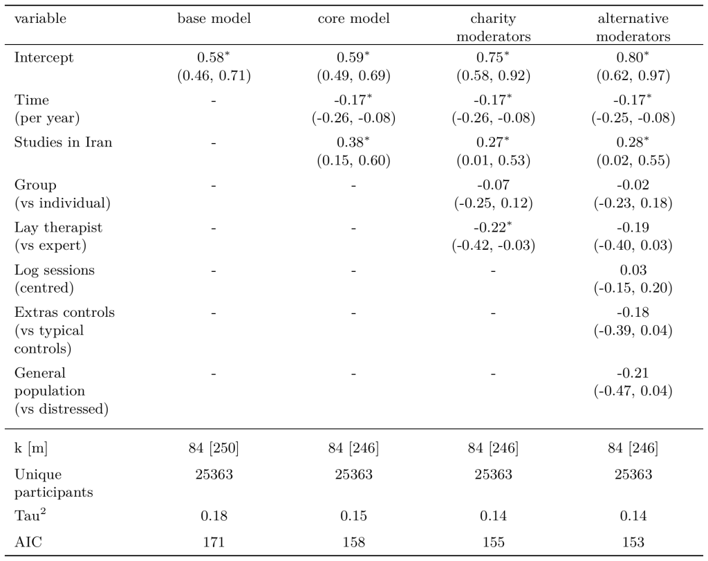
Note. All the effects presented above the first separation line are coefficients from the meta-analysis model. Their effects are in Hedge’s g (SD changes). The parentheses represent 95% confidence intervals. Statistical significance is represented such that * p < 0.05; ** p < 0.01; *** p < 0.001.
G2. Dosage
Dosage can be understood in two parts: intended number of sessions and actual attendance. For example, StrongMinds intended for participants to have 6 sessions, but participants attended on average 5.63 sessions, which is an attendance rate of 5.63/6 = 94%. In our general meta-analysis the average number of sessions intended is 7.18 and the attendance rate is 71%.
In Appendix G2.1 we discuss how to model intended sessions. In Appendix G2.2 we discuss how to model attendance. In Appendix G2.3 we discuss how to calculate the dosage adjustment.
G2.1 Modelling intended sessions dosage
We include intended numbers of sessions as a moderator in our model. We test both the log dosage (ln(sessions)) and the linear dosage. We also test if dosage interacts with follow-up time.
For continuous moderators like dosage, we include it in our model as mean-centred. Namely, we subtract the mean number of sessions to each session number so that it is 0 if it is equal to the average dosage. This is so it does not affect the interpretability of the intercept; namely, it remains comparable to other models where the intercept is the effect for the average dosage instead of interpreting an intercept where dosage is zero.
See Table G2 for the results.
Table G2: Modelling dosage.
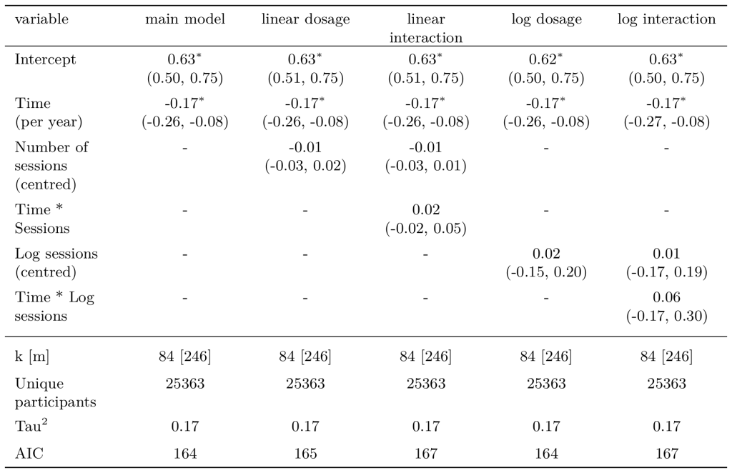
Note. All the effects presented above the first separation line are coefficients from the meta-analysis model. Their effects are in Hedge’s g (SD changes). The parentheses represent 95% confidence intervals. Statistical significance is represented such that * p < 0.05; ** p < 0.01; *** p < 0.001.
No effect of dosage is significant, and no interaction is significant. Cuijpers et al. (2013) also found a small, non-significant effect of the number of sessions in their analysis. The effect of dosage in this model is so small that taken at face value it would suggest that receiving 1 session has an initial effect that is 92% the value of receiving 10 sessions in a log model. This is surprising but there is research suggesting that single-session interventions can be impactful (see Appendix H for more discussion of those studies).
Note that the effect of dosage is small, non-significant, and negative in the linear model. It becomes small, non-significant, and positive if we remove the one study that has 32 intended sessions (Maselko et al., 2020) because it was a longterm follow-up of a study that involved giving participants 18 booster sessions – we think it is appropriate to remove for this analysis. Otherwise, the modelling does not change much (see Table G3). We illustrate these dose-response relationships in Figure G1.
Table G3: Modelling dosage (removing extreme study with 32 intended sessions).
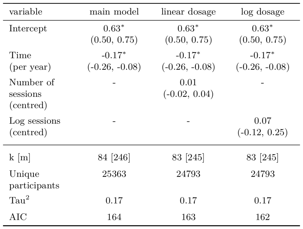
Note. All the effects presented above the first separation line are coefficients from the meta-analysis model. Their effects are in Hedge’s g (SD changes). The parentheses represent 95% confidence intervals. Statistical significance is represented such that * p < 0.05; ** p < 0.01; *** p < 0.001.
Figure G1: Dose-response relationship in our meta-analysis.
Note. The lines represent predictions from different models at post-intervention (the initial effect). The blue line represents the linear dose-response models. The orange line represents the concave (log) dose-response models. The dotted lines represent those models without the extreme study with 32 intended sessions. The dashed horizontal line represents effects of 0. The dashed vertical line is the average number of sessions.
G2.2 Modelling attendance
Ultimately, dosage refers to the intensity and quality of a treatment, so it is only fuzzily represented by the number of sessions intended. Ideally we would incorporate other information such as attendance. Namely, intending one session and participants attending one session is different from intending six sessions and participants attending only one of them. Therefore, we think it is an additional source of concern if we are comparing the intentional and unintentional receipt of only a few sessions.
For example, Friendship Bench intends a maximum of 6 sessions, but participants, in practice, attend 1.12/6 = 19% of sessions. It would be conceivable, and ideal, to apply one adjustment to account for the difference in intended sessions, and a second adjustment to account for the difference in attended sessions.
To model ‘attendance’, we tried to extract the average percentage of sessions attended in all the RCTs, but studies rarely report this information and often do so in inconsistent ways. We could only extract this information for 17 of our 84 studies (65 effect sizes), with an (unweighted) average percentage of sessions attended being 71% (range: 43% to 95%). This includes Barker et al. (2022), the largest study in the meta-analysis (n = 7,330), with an average percentage of sessions attended of 74%. This suggests that, in general, the RCTs we use do not have complete attendance either, so the number of sessions intended is also just a proxy for the actually attended sessions in the RCTsThis is still substantially more than the 19% attendance from Friendship Bench recipients. Note that StrongMinds has an average percentage of sessions attended of 5.63/6 = 94%, which is more than in these 14 studies (and more than the 76% in Baird et al., 2024), here, the adjustment would be an increase rather than a discount if we applied it..
We try to model attendance with just these 14 studies. We find a tiny and surprising non-significant prediction that more attendance (in percentage point) leads to less effect (and a strange non-significant interaction with intended sessions; see Table G4). This does not provide good grounds for an adjustment.
Table G4: Modelling attendance in the general meta-analysis.
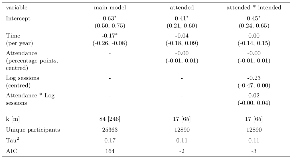
Note. All the effects presented above the first separation line are coefficients from the meta-analysis model. Their effects are in Hedge’s g (SD changes). The parentheses represent 95% confidence intervals. Statistical significance is represented such that * p < 0.05; ** p < 0.01; *** p < 0.001.
Alternatively, in the 2023 pre-post data Friendship Bench shared with us we can model a significant effect of the number of sessions attended in a simple linear regression. We find that the pre-post decline in mental health symptoms participants experience – as reported on the SSQ-14 scale (a 14-point scale) – is significantly predicted by the number of sessions (either linear or log) or the attendance rate (in percentage point). Namely, more attendance leads to a larger decline in depression (see Table G5).
Table G5: Modelling attendance in the Friendship Bench pre-post data.
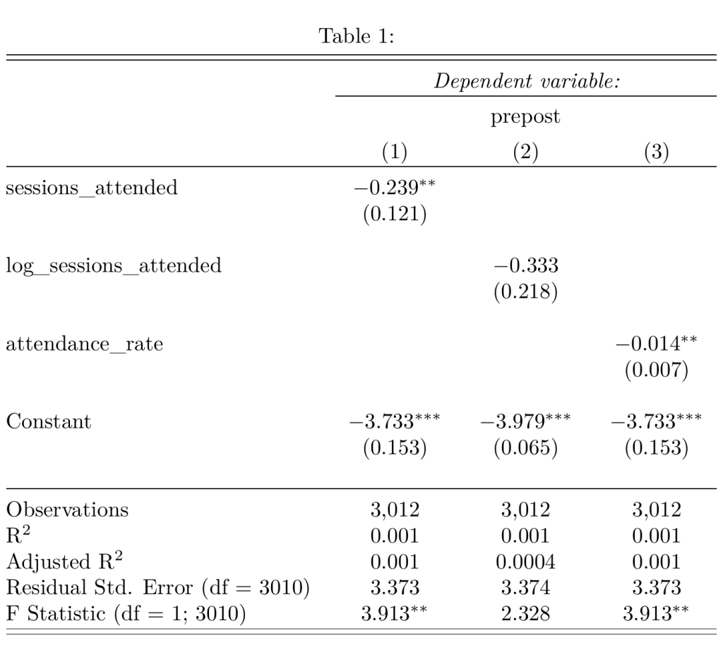
Note. The parentheses represent SE. Statistical significance is represented such that * p < 0.05; ** p < 0.01; *** p < 0.001.
G2.3 Different options for modelling the dosage adjustment
This leaves us with many options of how to model dosage by combining an intended sessions adjustment and an attended sessions adjustment. We present the options below with the dosage of Friendship Bench compared to the dosage in the general meta-analysis of psychotherapy in LMICs, but this applies to the other sources of evidence and to StrongMinds as well.
G2.3.1 General calculations
The first option is to split these two adjustments as one adjustment for the intended 6 sessions of psychotherapy from Friendship Bench and the 1.12/6 = 19% attendance rate from Friendship Bench and compare each element to their respective element in the meta-analysis to make an adjustment.
For the intended sessions adjustment we can compare it to the meta-analysis using information from our modelling as we do in our main analysis: Either with the log or the linear modelling of intended sessions (see Appendix G2.3.2). If one wanted to ignore this information they could do simple calculations of the dosage such as 6/7.18 for a linear adjustment or ln(6+1)/ln(7.18+1) for the log adjustmentWe add a constant of one to each side because ln(1) = 0, which means that by “+1” our adjustment can have the intuitive property of only being given a full discount when no sessions are actually attended (i.e., ln(0+1) = 0). Otherwise, it would imply that zero effect is represented by one session, which is implausible. See Section 5.2.2 for more detail..
The adjustment for attendance does not have as good an empirical backing as the one for intended sessions. We could calculate it as (-3.73 + -0.01 * 19%) / (-3.73 + -0.01 * 71%) = 0.84 for the attendance model with Friendship Bench pre-post data. We would not use the model from the general meta-analysis because the sign of the attendance predictor is counterintuitive. It could also be a simpler adjustment based on the rates in each data source such as: 19%/71%. Or it could be more simpler calculations about attendance either 1.12/6 = 0.19 for linear or ln(1.12+1)/ln(6+1) for log.
The second option would be to mix the two adjustments into one. One more conservative approach is to compare the attended sessions from the charity – 1.12 for Friendship Bench – to the intended sessions in the source (7.18 in the meta-analysis). The adjustment can be calculated with the log or the linear modelling of intended sessions (see Appendix G2.3.2) or with simpler calculations. If one wanted to ignore more information they could do simple calculations of the dosage such as 1.12/7.18 for a linear adjustment or ln(1.12+1)/ln(7.18+1) for the log adjustmentWe add a constant of one to each side because ln(1) = 0, which means that by “+1” our adjustment can have the intuitive property of only being given a full discount when no sessions are actually attended (i.e., ln(0+1) = 0). Otherwise, it would imply that zero effect is represented by one session, which is implausible. See Section 5.2.2 for more detail.. A more generous alternative – that can be used both in calculations or modelling – is to compare the attended sessions from the charity – 1.12 for Friendship Bench – to the intended sessions in the source (7.18 in the meta-analysis) adjusted for attendance in the source (7.18 * 71 = 4.95).
G2.3.2 Calculating the adjustment from the moderator in the meta-analysis and what we choose instead
Ideally, we would model the dosage adjustments (either mixed or just for intended sessions) using our moderator models. See Table G6 for the models we would use to do so. We explain how we would calculate the moderator adjustment (see Appendix G2.2) and dosage adjustment if we used such models:
- To calculate the moderator adjustment we calculate an initial effect (by setting the effect of time to 0) with the moderator model by setting each characteristic according to the charity. Taking Friendship Bench for the general prior for example, we set the dosage to ln(1.12)-ln(average sessions)The dosage variable is mean centred in order to keep the intercept and other covariates interpretable, so this is how we need to enter it back in. The results are the same as if we had not mean centred it and adding dosage in the simple manner of ln(sessions). If we use the charity-related RCTs we compare to the intended number of studies in the RCTs (in this case 6)., the group to 0 (this is set to 1 for StrongMinds), lay therapist to 1. This can then be calculated as 0.76 (intercept) + -0.17 * 0 (set time to 0 to get initial effect) + 0.24 * 0 (not Iran) + 0.09 * -1.74 (dosage) + -0.05 * 0 (not group therapy) + -0.24 * 1 (lay therapist) = 0.36. Then to get the adjustment we compare it to the initial effect of the main model: 0.36 / 0.59 = 0.62.
Because dosage is a really important moderator, we want to extract out the impact of dosage, separately from the other moderators. To do this, we calculate an initial effect with zero effect of dosageNamely, zero, which is the mean dosage in our model because dosage is mean-centred, see previous footnote. and an adjustment with just the other moderators 0.50 / 0.59 = 0.85. And then we extract out the effect of only dosage 0.62 / 0.85 = 0.73.
Table G6: Charity moderator models with dosage included (excluding study with 32 intended sessions)
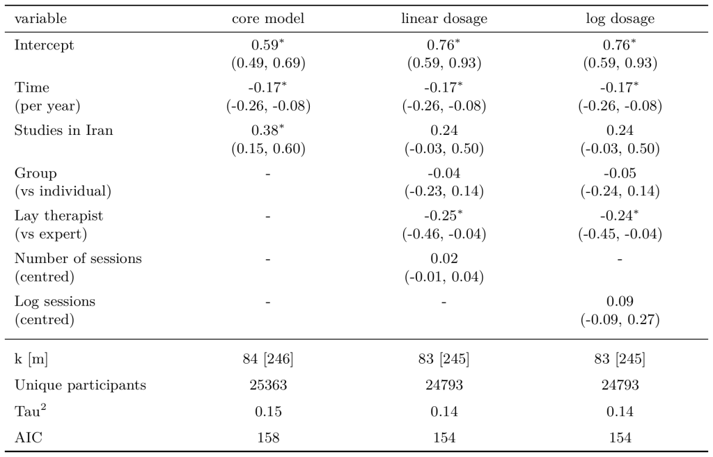
Note. All the effects presented above the first separation line are coefficients from the meta-analysis model. Their effects are in Hedge’s g (SD changes). The parentheses represent 95% confidence intervals. Statistical significance is represented such that * p < 0.05; ** p < 0.01; *** p < 0.001.
The issue is that the intended sessions coefficient has changed a lot through different iterations of this analysis (see Table G7), even though the other moderators or estimates in our analysis have not changed as much. This suggests to us that this is not a very stable and reliable predictor. Currently, it is very small and non-significant.
Table G7: How the intended sessions coefficient has changed across versions of the analysis.
|
Version 1 (2021) |
Version 2 (2022) |
Version 3 (2023) |
Version 3.5 (2024) |
Version 4 (2024) |
|
|
Dosage predictor (with only follow-up time as a covariate) |
Not evaluated |
Not evaluated |
0.04 (-0.15, 0.22) SDs per log session |
0.23 (0.01, 0.46) SDs per log session |
0.02 (-0.15, 0.20) SDs per log session 0.07 (-0.12, 0.25) SDs per log sessions [after removing study with 32 intended sessions] |
Instead of concluding that there is no effect of dosage, we use a calculation for the dosage adjustment that is more stable, where we assume a logarithmic dose-response relationship. This would be ln(attended sessions in the charity + 1) / ln(intended sessions in the source + 1). This is more conservative – and closer to the adjustments previously used – than if we used the moderator model.
G2.3.3 Summaries of the calculations
We summarise these different methods in Tables G8 and G9. The method we select (mixing intended and attended with log simple calculations) is fairly middle of the road, even somewhat conservative (in blue in the tables).
For our sensitivity analysis we select a more stringent and more favourable dosage adjustment (see Appendix O). The more stringent method we select for our sensitivity analysis is based on simple linear calculations (in red in the tables), while the more favourable method we select is simply no adjustment. This is the very upper bound of the possible effect, in relation to dosage.
There are some methods that can lead adjustments that suggests increases in effect, but these are in the case of StrongMinds which has higher attendance (94%) than in the general meta-analysis (71%), and so we do not select this for our sensitivity analysis.
Table G8: Potential dosage adjustments (ordered by dosage adjustment size) for Friendship Bench general prior.
|
Dosage Adjustment |
Mixed Adjustment |
Intended Sessions Adjustment |
Attendance Adjustment |
|
0.94 |
Linear Moderator Model: Attended sessions vs attendance-adjusted (7.18 * 71%) intended sessions (0.94) |
||
|
0.83 |
Log Moderator Model: 0.99 |
FB Pre-post Attendance Model: 0.84 |
|
|
0.81 |
Linear Moderator Model: Attended sessions vs intended sessions (0.81) |
||
|
0.73 |
Log Moderator Model: Attended sessions vs attendance-adjusted (7.18 * 71%) intended sessions (0.73) |
||
|
0.69 |
Log Moderator Model: Attended sessions vs intended sessions (0.69) |
||
|
0.42 |
Simple Log: Attended sessions vs attendance-adjusted intended sessions (ln(1.12 + 1) / ln(7.18 * 71% + 1)) |
||
|
0.38 |
Log Moderator Model: 0.99 |
Simple Log Attendance: ln(1.12 + 1) / ln(6.00 + 1) = 0.39 |
|
|
0.36 |
Simple Log: ln(6.00 + 1) / ln(7.18 + 1) = 0.93 |
Simple Log Attendance: ln(1.12 + 1) / ln(6.00 + 1) = 0.39 |
|
|
0.36 |
Simple Log: ln(1.12 + 1) / ln(7.18 + 1) |
||
|
0.22 |
Simple Linear: Attended sessions vs attendance-adjusted intended sessions (1.12/(7.18 * 71%)) |
||
|
0.18 |
Linear Moderator Model: 0.95 |
Simple Linear Attendance: 1.12/6.00 = 0.19 |
|
|
0.16 |
Simple Linear: 6.00/7.18 = 0.84 |
Simple Linear Attendance: 1.12/6.00 = 0.19 |
|
|
0.16 |
Simple Linear: 1.12/7.18 |
Table G9: Potential dosage adjustments (ordered by dosage adjustment size) for StrongMinds general prior.
|
Dosage Adjustment |
Mixed Adjustment |
Intended Sessions Adjustment |
Attendance Adjustment |
|
1.11 |
Simple Linear: Attended sessions vs attendance-adjusted intended sessions (5.63/(7.18 * 71%)) |
||
|
1.06 |
Log Moderator Model: 0.99 |
FB Pre-post Attendance Model: 1.07 |
|
|
1.05 |
Simple Log: Attended sessions vs attendance-adjusted intended sessions (ln(5.63 + 1) / ln(7.18 * 71% + 1)) |
||
|
1.02 |
Log Moderator Model: Attended sessions vs attendance-adjusted (7.18 * 71%) intended sessions (1.02) |
||
|
0.99 |
Linear Moderator Model: Attended sessions vs attendance-adjusted (7.18 * 71%) intended sessions (0.99) |
||
|
0.98 |
Log Moderator Model: Attended sessions vs intended sessions (0.98) |
||
|
0.96 |
Log Moderator Model: 0.99 |
Simple Log Attendance: ln(5.63 + 1) / ln(6.00 + 1) = 0.97 |
|
|
0.94 |
Linear Moderator Model: Attended sessions vs intended sessions (0.94) |
||
|
0.90 |
Simple Log: ln(6.00 + 1) / ln(7.18 + 1) = 0.93 |
Simple Log Attendance: ln(5.63 + 1) / ln(6.00 + 1) = 0.97 |
|
|
0.90 |
Simple Log: ln(5.63 + 1) / ln(7.18 + 1) |
||
|
0.89 |
Linear Moderator Model: 0.95 |
Simple Linear Attendance: 5.63/6.00 = 0.94 |
|
|
0.78 |
Simple Linear: 6.00/7.18 = 0.84 |
Simple Linear Attendance: 5.63/6.00 = 0.94 |
|
|
0.78 |
Simple Linear: 5.63/7.18 |
G3. Other moderators
G3.1 Expertise and group or individual delivery format
We are interested in how cost-saving methods – using non-experts and group delivery – affect psychotherapy's effectiveness. In LMICs, the shortage of mental health specialists limits access. Task-shifting, where non-experts are trained by experts (Galvin & Byansi, 2020), and group therapy are two approaches that reduce costs and expand reach.
Expertise is whether the deliverer was someone with formal training in psychotherapy (e.g., at least an undergraduate degree) or if they were a peer or community health worker trained by an expert to deliver the training. See Table G10 for a distribution (note that we combine the ‘unclear but probably experts’ with those who were clearly expert to make a simple comparison in the model). Having a non-expert deliverer significantly reduces the effect, see Table G11 for the models. This is consistent, albeit less stringent than, with the results of Venturo-Conerly et al.’s (2023) meta-analysis of the effect of psychotherapy on youth, which found a much larger effect from clinicians (g = 1.59) than lay providers (g = 0.53).
Table G10: Distribution of expertise.
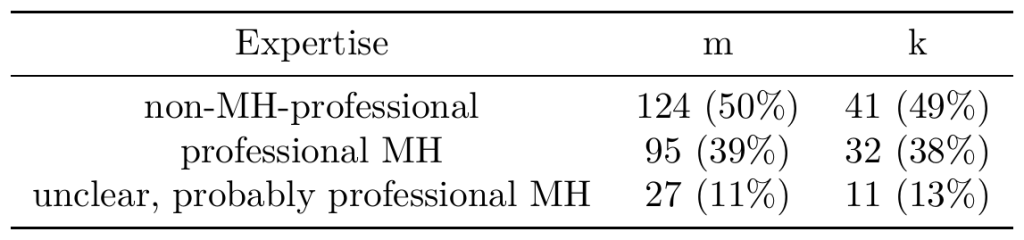
Table G11: Modelling expertise.
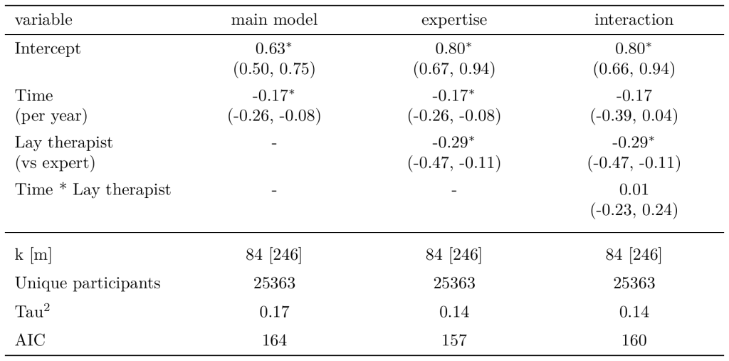
Note. All the effects presented above the first separation line are coefficients from the meta-analysis model. Their effects are in Hedge’s g (SD changes). The parentheses represent 95% confidence intervals. Statistical significance is represented such that * p < 0.05; ** p < 0.01; *** p < 0.001.
Delivery is whether the psychotherapy was delivered to individuals or to groups (see Table G12 for a distribution). We find that using group delivery does not lead to a significant decrease in the effectiveness of psychotherapy compared to individual delivery (see Table G13 for the modelling). Cuijpers and colleagues, in contrast to our results, found group delivery to have higher effects in their meta-analyses of psychotherapy in LMICs (Cuijpers et al., 2018; Tong et al., 2023). We are unsure what explains this difference.
Table G12: Distribution of delivery.
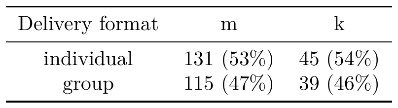
Table G13: Modelling delivery.
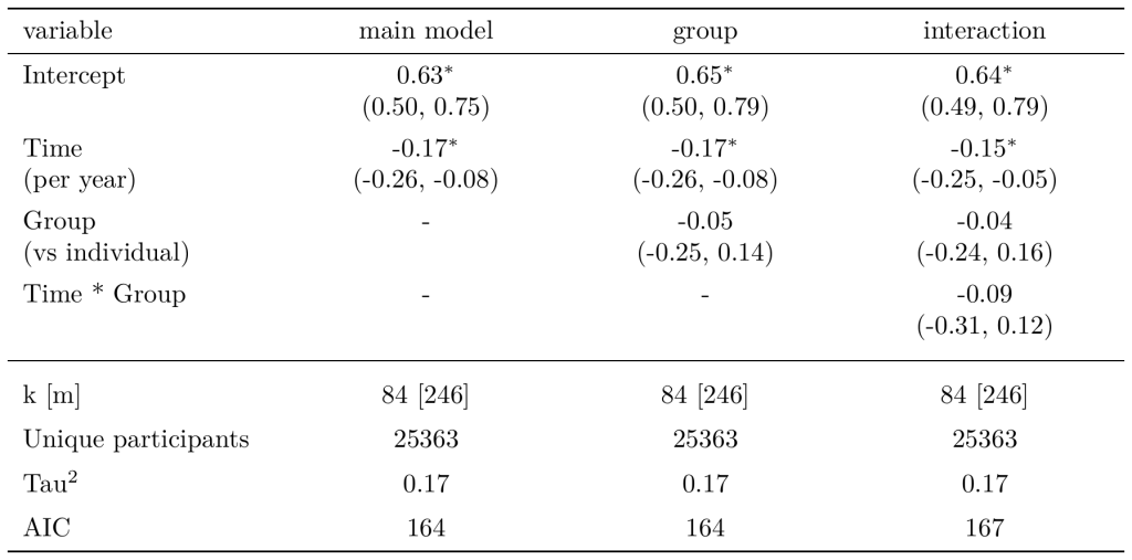
Note. All the effects presented above the first separation line are coefficients from the meta-analysis model. Their effects are in Hedge’s g (SD changes). The parentheses represent 95% confidence intervals. Statistical significance is represented such that * p < 0.05; ** p < 0.01; *** p < 0.001.
G3.2 Control group
Control group types can affect results. In general we are interested in control groups types where participants receive the equivalent of nothing new (usual care, treatment as usual, wait-list, etc.). Because receiving nothing new will best represent the counterfactual effect of providing psychotherapy to individuals who have little access to psychotherapy otherwise. Note that in most cases, studies are often vague about what “treatment as usual” entails, so we assume it represents the local standard of care. As we mentioned in Section 1, we expect the local standard of care to be low in most cases because the amount of cases of depression and anxiety that receive adequate treatment in LMICs is between 2-3% (Alonso et al., 2018; Moitra et al., 2022).
See Table G14 for a distribution of effects according to the different control groups we find. See Table G15 for modelling of the effect of control group type. We consider Enhanced Usual Care (EUC; the standard treatment or care that has been augmented with additional elements) and active controls, (AC; control groups that receive some form of treatment designed specifically to be compared with the experimental treatment but is not expected to have a therapeutic effect) as ‘controls with something extra’, because the control group is provided with something more than if they had not participated. Extra control groups have non-significantly lower effects than the other typical control groups.
Table G14: Distribution of control group type.
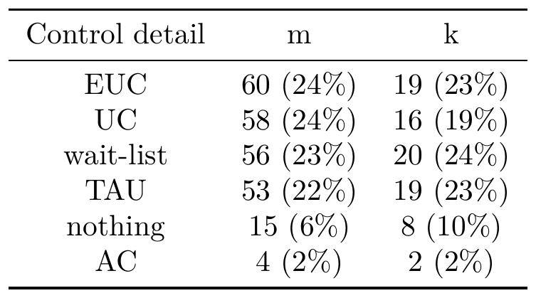
Table G15: Modelling control group type.
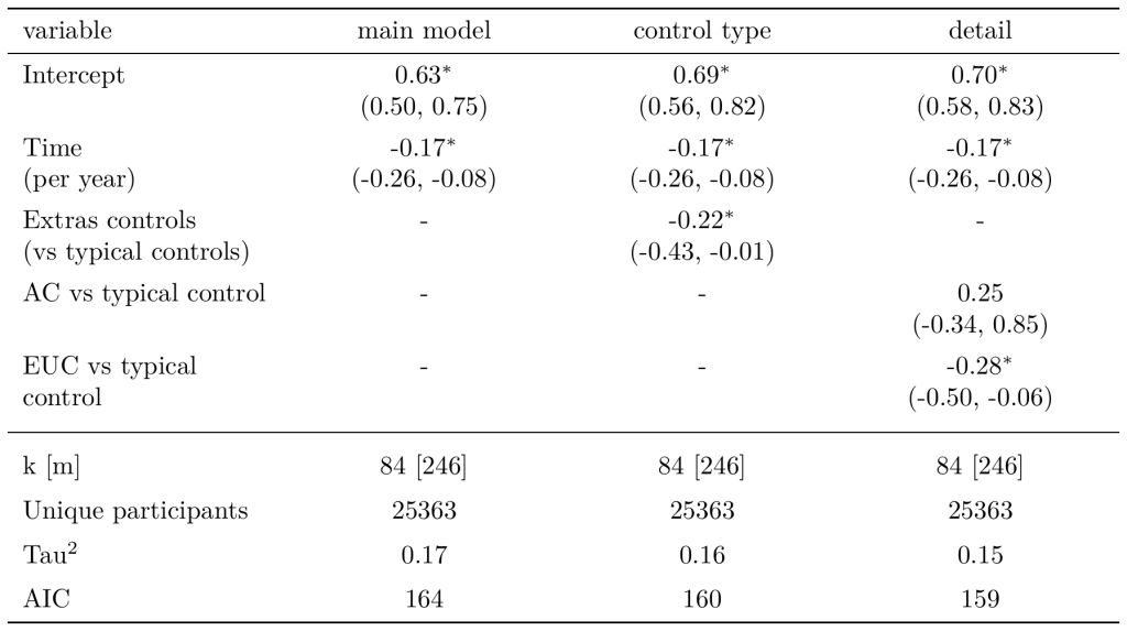
Note. All the effects presented above the first separation line are coefficients from the meta-analysis model. Their effects are in Hedge’s g (SD changes). The parentheses represent 95% confidence intervals. Statistical significance is represented such that * p < 0.05; ** p < 0.01; *** p < 0.001.
G3.3 Medical population
There are different target populations in our data (see Table G16). The majority of our data’s population is composed of individuals who pass a threshold of mental distress (e.g., being treated for depression). However, some interventions (e.g., Haushofer et al., 2020) deliver psychotherapy to the general population (i.e., not mentally distressed). We find a non-significant decline in effectiveness when psychotherapy is delivered to the general population (versus a distressed population; see Table G17).
Table G16: Distribution of target population.
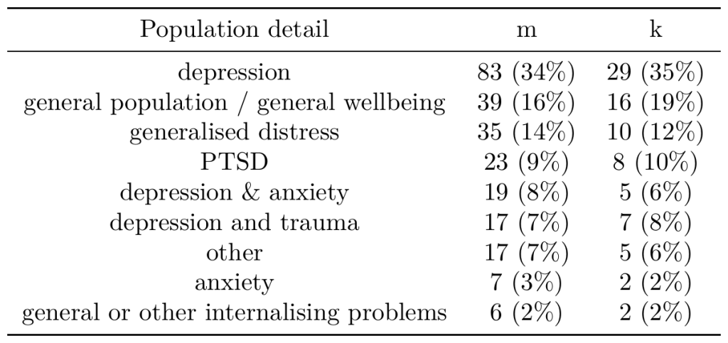
Table G17: Modelling target population.
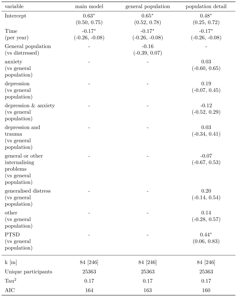
Note. All the effects presented above the first separation line are coefficients from the meta-analysis model. Their effects are in Hedge’s g (SD changes). The parentheses represent 95% confidence intervals. Statistical significance is represented such that * p < 0.05; ** p < 0.01; *** p < 0.001.
G3.4 Baseline effects
We try to model whether baseline wellbeing levels moderate the benefits of psychotherapy (i.e., whether the more depressed/anxious groups benefit from psychotherapy more). We operationalise baseline level as the proportion (0-100%) of the maximum on the wellbeing scale used that the treatment group average represents (e.g., a score of 7 on a 0-10 scale will represent 70% at baseline). We frame this negatively (by reversing positive scales) as more baseline level means more mental distress. This is limited because we are using a meta-analysis where we are comparing the effect of baseline levels between studies and not between participants, and we lack causal identification. Nevertheless, we think this is informative considering this is a topic we struggle to find clear answers to in the literature.
The average baseline level is 48% (range 6% to 83%). We could not calculate baseline levels for 30 effect sizes. See Figure G2 for the distribution of effect sizes.
Figure G2: Distribution of effect sizes across baseline level.
Note. The blue line represents a fitted smoothing curve (geom_smooth), with the grey area indicating the 95% confidence interval of the fit.
We modelled the effect of baseline levels in our meta-regression, addressing several causal modelling considerations using extracted data from each study. Specifically, we identified causal backdoors between baseline levels and intervention effects that should be controlled for (see Figure G3). Factors such as scale length, whether the scale is positively or negatively framed (i.e., whether higher scores indicate greater wellbeing or distress), and whether participants were selected based on a mental distress cut-off can influence both participants’ baseline and endline self-reports. To account for these influences, we included these variables as controls.
Figure G3: Causal modelling of baseline level.
Note. The nodes are: Baseline level (B), Effect (E), Scale length (L), Scale framing (F), and selected on a mental distress cut-off (C).
Additionally, we tested a quadratic term for baseline level and its interaction with follow-up time, but neither improved the model fit (based on AIC and log-likelihood tests) compared to a model with baseline and the control variables alone. Our findings indicate that a one percentage point increase in baseline level significantly improves the intervention effect by 0.005 SDs, suggesting that individuals with higher levels of distress benefit more from psychotherapy (see Table G18).
Table G18: Modelling baseline levels.
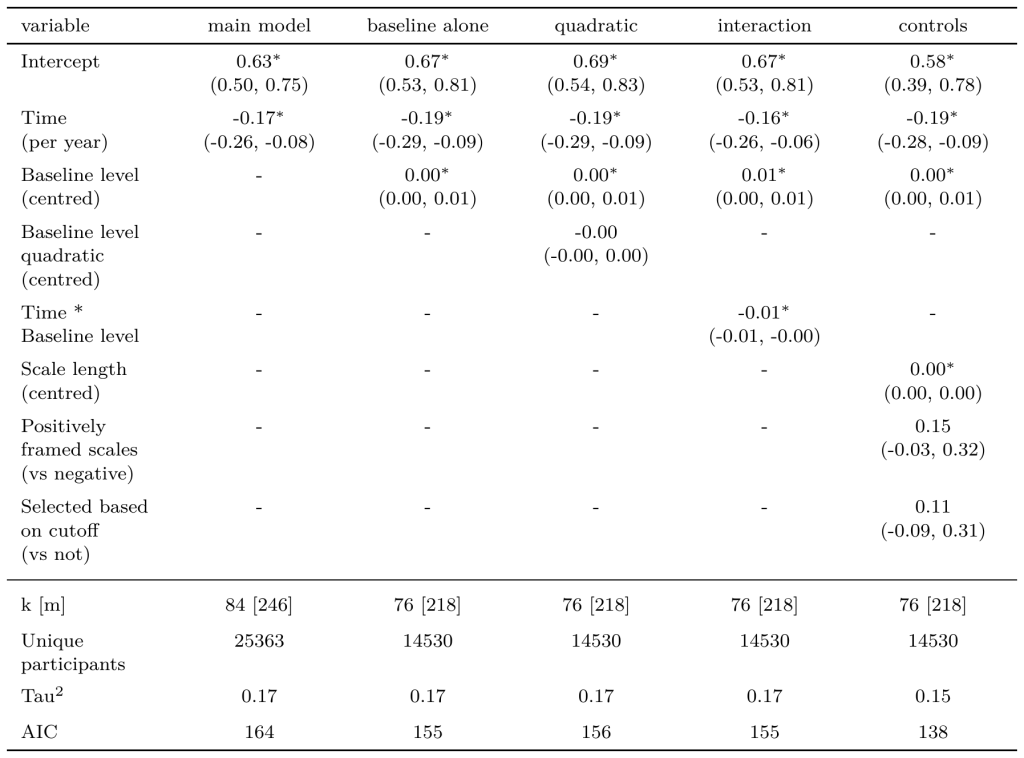
Note. All the effects presented above the first separation line are coefficients from the meta-analysis model. Their effects are in Hedge’s g (SD changes). The parentheses represent 95% confidence intervals. Statistical significance is represented such that * p < 0.05; ** p < 0.01; *** p < 0.001.
G3.5 Outcome types
Outcome types could change the size of the effect (e.g., maybe participants report greater changes on a life satisfaction question than a depression question), but we did not expect it to matter. Our main interest is subjective wellbeing (SWB; 9% of effect sizes) measures but the majority of our effect sizes (91%) are on affective mental health (MHa) outcomes (see Table G19). There are no significant differences between the types of measures (see Table G20). We treat them as 1:1 equivalents. See Dupret et al. (2024) for more discussion about combining SWB and MHa measures.
Table G19: Distribution of outcome types.
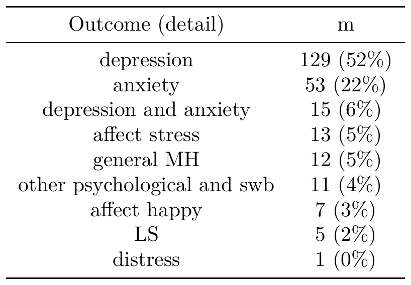
Table G20: Modelling outcome types.
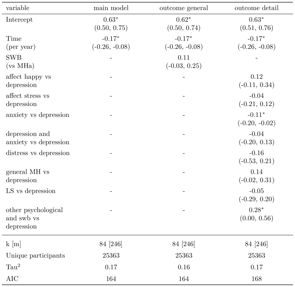
Note. All the effects presented above the first separation line are coefficients from the meta-analysis model. Their effects are in Hedge’s g (SD changes). The parentheses represent 95% confidence intervals. Statistical significance is represented such that * p < 0.05; ** p < 0.01; *** p < 0.001.
G3.6 Modalities
We classify the different modalities (types of psychotherapy) in the studies we have extracted (see Table G21). A few studies were hard to classify so we group them as “others”. We find no significant difference between CBT (one of the most popular modalities) and the other modalities (see Table G22). Previous meta-analyses also found limited evidence supporting the superiority of any one form of psychotherapy for treating depression (Cuijpers et al., 2020c; Cuijpers et al. 2021, Cuijpers et al. 2023).
Table G21: Distribution of modalities.
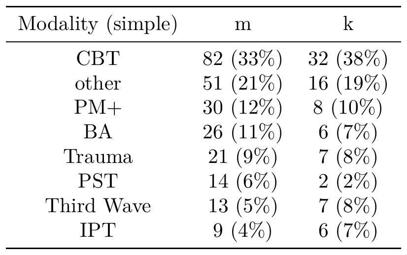
Table G22: Modelling modalities.
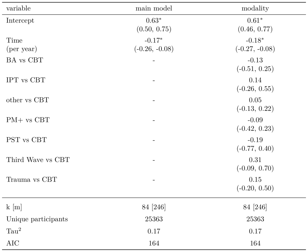
Note. All the effects presented above the first separation line are coefficients from the meta-analysis model. Their effects are in Hedge’s g (SD changes). The parentheses represent 95% confidence intervals. Statistical significance is represented such that * p < 0.05; ** p < 0.01; *** p < 0.001.
We did not include modality (CBT, IPT, etc.) as a moderator in our charity moderator model for the validity adjustments because: (1) this model depends on us determining which modalities different studies belong to (many of which have hard to classify modalities), (2) most of the coefficients are imprecisely estimated, and (3) most of the evidence for PST, the modality for Friendship Bench, comes from the Friendship-Bench-related RCTs themselves, which would be too much like double counting. Considering IPT has a non-significant higher effect than CBT, including this moderator would have likely increased the effect of StrongMinds.
G3.7 Other participant characteristics
We extracted whether the population of a study was targeted for (or simply contained) high levels of the following characteristics: HIV, cancer, being in a perinatal situation, interpersonal violence, or were refugees. We found very few of these across the effect sizes (see Table G23) and none of them significantly moderate the effect of psychotherapy (see Table G24).
Table G23: Distribution of other characteristics.
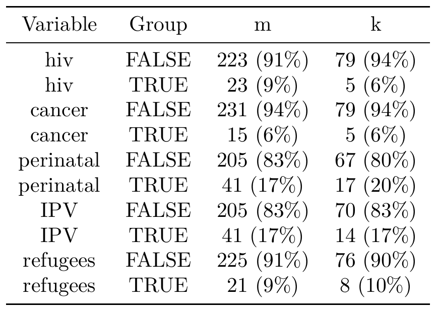
Table G24: Modelling other characteristics.
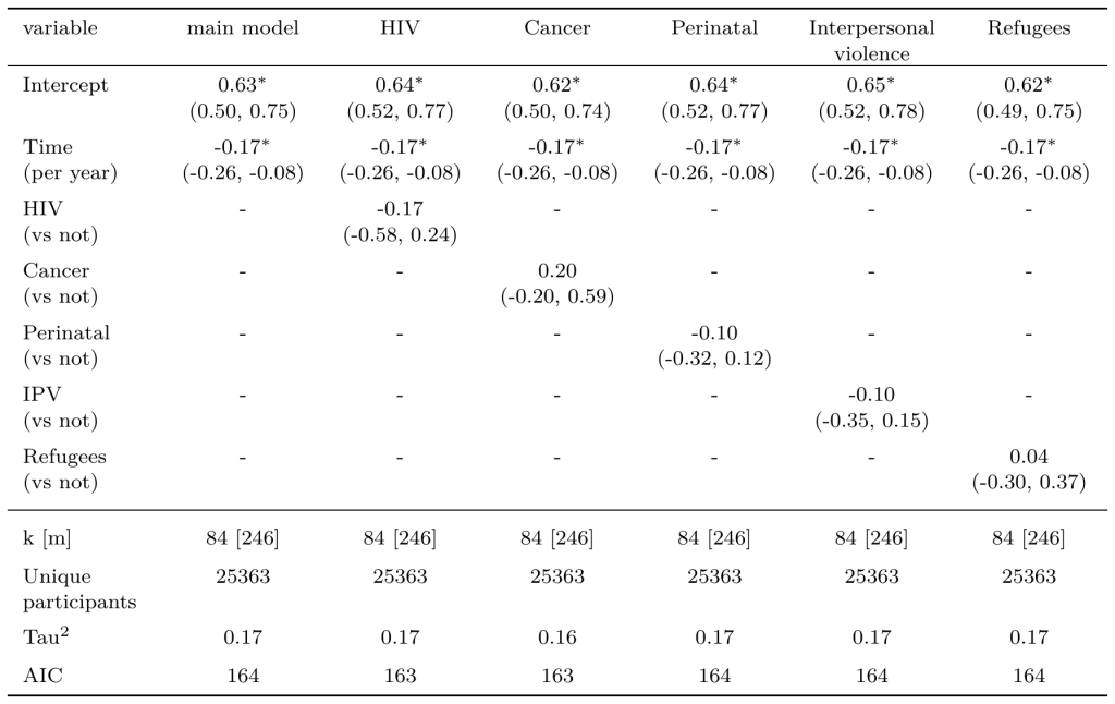
Note. All the effects presented above the first separation line are coefficients from the meta-analysis model. Their effects are in Hedge’s g (SD changes). The parentheses represent 95% confidence intervals. Statistical significance is represented such that * p < 0.05; ** p < 0.01; *** p < 0.001.
G4. Combining and selecting moderators
In Table G25, we present all the different moderator models we consider. Two models we have presented before:
- The core model is our general model with moderation for time and bias from Iran, as selected in Section 4.1.
- The charity moderators is the model where we select moderators based on theory to determine which characteristics of the charities we want to adjust for in our external validity adjustments (see Section 5.2).
- The full model select model is a model that selects any predictor in addition to those of the core model that significantly increased model fit according to the AIC values and the loglik test. Note that we do not select this model but present it for the interested reader. We think theory and causal understanding are too important for this sort of model to be selected.
Table G25: Different overall models.
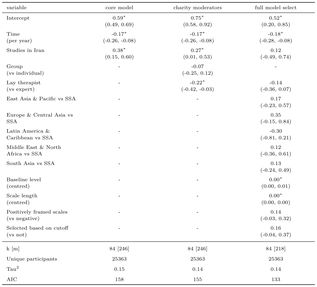
Note. All the effects presented above the first separation line are coefficients from the meta-analysis model. Their effects are in Hedge’s g (SD changes). The parentheses represent 95% confidence intervals. Statistical significance is represented such that * p < 0.05; ** p < 0.01; *** p < 0.001.
Appendix H: Discussing Friendship Bench dosage
We summarised the main reasons why it is not implausible that Friendship Bench’s low dosage could still be effective in Section 5.2.3 of the main text. In the sections below, we explain these reasons in more detail.
H1. Severe adjustments
Even when we try more severe adjustments, based on a simple linear dosage assumption (1.12 / 7.18 = 0.16), rather than the concave dosage model from our moderator model, we find that the cost-effectiveness of Friendship Bench is still relatively high at 23 WBp1k (see Appendices G2 and O3 for more detail). This is about 3x more cost-effective than cash transfers. To be clear, in this linear adjustment, it is assumed that the first session is equally as effective as subsequent sessions. As discussed below, we think it is more likely that first sessions are more impactful.
H2. Effectiveness even with a few sessions
Is it plausible that so little as 1.12 sessions can still produce an effect? Potentially, yes. Research by Schleider and colleagues (Schleider & Weisz, 2017; Schleider & Beidas, 2022; Schleider et al., 2022; Fitzpatrick et al., 2023; see also Kim et al., 2023) suggest that psychotherapy can be effective even with one session.
In a large (50 studies and 299 effect sizes) meta-analysis of single-session mental health interventions for youth in HICs (looking at a wide array of interventions and common mental health disorders), Schleider and Weiss (2017) found effects of 0.32 SDs overall, 0.59 SDs on anxiety, and 0.21 SDs on depression. In an large (N = 2,452) RCT by Schleider et al. (2022), they find that an online 30min single-session intervention during COVID-19 for adolescents has an effect of 0.18 SDs.
Studies of the Shamiri programme (a mental health charity in Kenya) show benefits of single session psychotherapy as well. In an RCT of single-session positive psychotherapy in Kenya compared to an active control, participants experienced a decrease in anxiety symptoms of 0.31 SDs (but no significant change for depression symptoms; Venturo-Conerly et al., 2022). An earlier digital version of the same programme found benefits of 0.50 SDs for depression and 0.83 SDs for anxiety (Osborn et al., 2020).
The context of these studies is not exactly that of Friendship Bench – notably because they are about adolescents – but still these effect sizes are similar to the initial effectIt is more comparable to compare the initial effect than the total effect after integration over time. of the general prior after the dosage adjustment: 0.59 * 0.36 = 0.21 SDs. This suggests that our adjustment might be functioning appropriately.
Nevertheless, even if a few sessions can be effective, we think it is relevant whether the programme is designed to work as a single session compared to being designed to work over multiple sessions. Namely, intending one session and participants attending one session is different from intending six sessions and participants attending only one of them. Therefore, we think it is an additional source of concern if we are comparing the intentional and unintentional receipt of only a few sessions. Note that our adjustment is already mixing concerns of intended and attended sessions (see Appendix G2.3 for more detail), and so this concern is accounted for. However, is it plausible that unintentionally low attendance can be effective? We have a clustering of small reasons that make us think it might be.
We think that general understanding about mental health problems is much lower in LICs, which is supported by the sparse provision of mental health treatment in LICs and some of the treatment provided can be actively harmful, such as chains (Walker et al., 2021; Moitra et al., 2022). Therefore, the first few sessions of a psychotherapy course could play an important psycho-educational role and thereby carry an important effect in a few sessions (or even one session) – more so than they would in high-income countries where we have relatively more awareness. If one has little understanding of why one is experiencing the terrible internal issues that come from depression or anxiety, or even attributes it to demons or curses, discovering that this is a treatable medical condition and that they are not on their own could be an immense source of relief. One of the authors (Michael Plant) conducted site visits (see Section 9.4) to both charities. He spoke to past and former clients, some of whom reported they had ‘no idea’ about mental health before. He also spoke to StrongMinds staff who mentioned that clients often think that poor mental health is due to being cursed.
Friendship Bench shared with us their manual for their lay health workers. There is a strong emphasis on psychoeducation (e.g., “It is important to know that depression can be treated!”). Furthermore, the first session is not just an introductory session but very much a full session where a cycle of problem solving is applied:
- Client shares what is going on in their life, the counsellor listens empathically and makes a list of problems the client faces.
- They choose a problem, set goals, and brainstorm solutions.
- They focus on detailed solutions and devising an action plan.
- The client is invited to join a peer support group.
Subsequent sessions review how the action plan went. If it went well, another problem can be addressed. If it did not go well, more solutions are explored. Overall, this lends some plausibility to one session being effective by itself. Thereby, providing 6 sessions is not necessarily the aim, but solving problems that affect clients’ mental health is. We consider 6 sessions to be the intended sessions as a conservative measure.
Furthermore, Friendship Bench provides support beyond just the sessions of psychotherapy via supplementary peer support groupsFriendship Bench also invites clients to join support groups to supplement the psychotherapy sessions. Is it possible that Friendship Bench has a higher attendance if we count support groups? We think this is unlikely. Friendship Bench reports in their 2023 annual review (p. 12), there are now 578 groups with a total of 6,294 clients. Given that Friendship Bench reported seeing 214,020 clients in 2023, the number of clients attending support groups would only constitute about ~3% of the total. So, we do not make any upwards adjustments in our analysis to account for the potential impact of these groups. . Friendship Bench has communicated to us that they also asked the sample of participants (n = 3,326) in the 2023 pre-post survey to self-report how many sessions they had attended, which was, on average, 2.01 sessions. This could be because recall is imperfect, but also because participants included informal meet-ups such as the suggested peer support groups or other informal meetings. While this suggests the actual dosage might be higher than 1.12 sessions, we have more uncertainty about the 2.01 figure, so we use the more conservative 1.12 sessions in our modelling.
In the 2023 M&E pre-post data that Friendship Bench shared with us (see Section 3.3.2), there was an average reduction in mental health symptoms of -4.13 points on the SSQ-14 and we estimate that the Friendship Bench M&E pre-post data alone has a cost-effectiveness of 14 WBp1k (see Section 7.3 and Appendix K)Note that the 1.12 average number of sessions attended for Friendship Bench clients comes from communications from Friendship Bench. In the pre-post data they shared with find an average number of sessions attended of 1.16 sessions. These slight differences come from trivial differences in the number of clients included in the data set.. Of course, we have uncertainties about our synthetic control methodology here and do not give this source of data all the weight (see Section 7). But this does support the idea that Friendship Bench’s programme can be effective even though the clients do not attend all the intended sessions. Additionally, Friendship Bench shared with us a dataset of 8,147 clients surveyed at baseline and at 6 weeks follow-up across the years 2021 to 2024 (which includes the 2023 clients mentioned above), the average reduction is very similar to the 2023 levels with -4.18 points on the SSQ-14 for a similar attendance levelIn the 2021-2024 data, we do not have the objective number of visits, but the self-report question gives an average of 1.97 sessions..
H3. Friendship Bench’s experience
Friendship Bench has communicated to us that the low attendance is not necessarily a worry because some clients only attend one session because they are satisfied that it sufficiently helped them and attending additional sessions is not needed nor obligatory (which may be a feature of problem solving therapy). Hence, this lends support to a few sessions being plausibly helpful. However, they have also told us that they plan to “offer more mobilization and stakeholder engagements for mental health awareness and uptake”. Improved attendance would be helpful for clients who might only attend one or few sessions because of barriers to therapy such as: transportation issues, rural socio-economic inhibiting factors, dependency syndrome where clients expect something more tangible as would be provided by typical humanitarian agencies, competing priorities in urban areas (e.g., fast paced lives), and highly mobile or in-transit populations. Additionally, if clients receive the psychotherapy as part of a wider integrated health service, they might stop attending once their other health problems are solved. It is unclear what is the proportion of clients who do few sessions because the sessions worked for them or because of barriers. These are issues that can be improved via implementation, and we are told that ongoing efforts in this domain are priorities for Friendship Bench.
Why does the attendance differ so much between StrongMinds and Friendship Bench when they both work with low-income clients in low-income countries? We do not know for sure, but there are a few aspects that could contribute – none of which we have yet to confirm empirically:
- IPT (which StrongMinds delivers) might be less likely to satisfy clients after only one or two sessions like PST (which Friendship Bench delivers), and so clients attend more IPT sessions.
- The group format delivered by StrongMinds (vs. the individual format delivered by Friendship Bench) might increase attendance by fostering bonding with others as well as social pressure to attend as their absence would be noticed.
- StrongMinds might have more systems in place to encourage attendance.
- StrongMinds might recruit clients who have fewer barriers to attendance (more local, where travel is easier/cheaper, etc.) than those recruited by Friendship Bench.
We hope that future funding for Friendship Bench enables them to improve attendance (for those in need, as some clients may only need a few sessions), which, we think, would improve their effectiveness, cost-effectiveness, and assuage our uncertainties.
Appendix I: Other validity adjustments
I1. Response bias
Responses on subjective wellbeing (SWB) and affective mental health (MHa) scales can be subject to response bias, a range of tendencies that cause participants to respond inaccurately to self-report questions. There are many such biases, but the main biases include:
- Demand Characteristics: Respondents may pick up on cues from the researcher or interviewer that suggest a particular response is expected or desired, influencing their answers. This is often referred to as Experimenter demand effects or “behavioral changes that result from participants shifting their response in reaction to an inference on the experimenter’s hypothesis” (De Quidt et al., 2019). Following Zizzo (2010) and Bandiera et al. (2018), we further split demand effects into two types:
- Social: Responding in line with what you believe to be the experimenter’s hypothesis to “help” the experimenter.
- Cognitive or material: Providing desirable responses to increase chances of receiving additional support for self or others.
- Social Desirability Bias: Respondents may answer questions in a way that they believe is socially acceptable or favourable, even if it does not reflect their true beliefs or behaviours.
- Acquiescence Bias: This occurs when respondents have a tendency to agree or say "yes" to questions, regardless of the content, leading to a bias toward agreement.
For most of our evaluations (psychotherapy, cash transfers, etc.), the response bias of concern is ‘demand characteristic’ because we are using results from RCTs of interventions. In many interventions, such as cash transfers or psychotherapy, it is difficult-to-impossible to blind participants to their condition, so participants receiving the treatment may be more likely to respond in a manner they expect to be beneficial socially or materially. This might include reporting higher scores on wellbeing measures in order to receive more treatment, or to improve the likelihood that the programme is deemed a success so others will receive treatment. We review some literature and estimate that demand characteristics can inflate results by a factor of 1.18, thereby, we should apply an adjustment of 1/1.18 = 0.85 (a 15% discount) to correct the results (see Appendix I1.1 for detail).
However, we only apply this adjustment to the M&E pre-post data (see below). We do not apply this adjustment to our causal estimates (e.g., general evidence and charity-related evidence) for the following reasons. We are very uncertain about our estimate. Calculating an empirical adjustment for response bias is not as straightforward (see footnote for an explanation of the challenges)One major challenge is determining whether to make a fixed adjustment (e.g., 0.25 SD) or relative adjustment (e.g. 10%). The decision depends on whether you model demand effects as uniform, with participants inflating their scores by a constant amount, or proportional, in which the size of the bias depends on the size of the true effect. We are uncertain which model is more appropriate. Another challenge is determining whether the available evidence is generalizable to the current context. . We hope we can form a better empirical estimate in the future as we find more data on the topic. Furthermore, this would affect all the charities we evaluate (StrongMinds, Friendship Bench, GiveDirectly, etc.) in plausibly similar ways. We do not think there would be strong deviations in response bias between psychotherapy, cash transfers, and other interventions we analyse. So, it would not change the relative differences and we would have to apply it to every analysisOur analysis of anti-malaria bednets (Plant et al., 2022) depends more on social desirability bias because it is primarily based on average levels of life satisfaction of individuals in the countries where AMF operates. Namely, it looks better to report higher wellbeing. We briefly tried to estimate this empirically and found an inflation of 1.09 or 0.92 (8% discount). This is smaller than the 0.85 adjustment for demand characteristics, but we think that, considering the uncertainty around these estimates, this still washes out across all analyses. To determine this adjustment we looked at three experiments where participants were randomised to be anonymously interviewed (and presumably less subject to social desirability bias than in typical survey conditions; Reisinger, 2022; Holford et al., 2015; Rosa, 2018; total sample size = 7,982). We also looked at an experiment that randomised participants to a truth telling exercise (Carlsson & Kataria, 2018; n = 1,700), which seems like a plausible lower bound of the magnitude of social desirability bias.. While we think this would be a useful addition to our methodology, we think we should wait to apply this adjustment broadly until we have better data on the topic.
We think estimates based on M&E data are more at risk for response bias than the RCT sources because the responders can plausibly connect the data collection process with the charity that has previously benefited them, and there may be organisational incentives to show positive outcomes. This seems like a reasonable precaution, especially in light of the high degree of speculation involved in our ‘pseudo-synthetic control’ methods for pre-post data (see Appendix K for more detail), and the fact that it represents a very small part of our final estimate.
I1.1 Details about demand characteristics
We review evidence relevant to RCTs and survey responses in general (experiments = 13, n = 32,545) and SWB measures in general (experiments = 4, n = 9,682). Of this, we are aware of three studies that have attempted to quantify the size of demand effects directly.
First, de Quidt et al. (2018) randomly assigned participants to receive a weak (signalling hypothesis) or strong (asking the participant) signal of the researcher’s hypothesis across 11 common experimental tasks online“We conduct seven online experiments with approximately 19,000 participants in total, in which we construct bounds on demand-free behavior for 11 canonical games and preference measures.” de Quidt et al. (2018, p. 3).
“Specifically, we study simple time, risk and ambiguity preference elicitation tasks, a real effort task with and without performance incentives, a lying game, dictator game, ultimatum game (first and second mover), and trust game (first and second mover). Our data come from US-based Amazon Mechanical Turk (MTurk) participants and a US nationally representative online panel.” de Quidt et al. (2018, p. 3).. In the subset of studies (k = 5) that compared the strong signal to a control group receiving no signal, the average bias was 0.25 SDsWe calculated this value by taking the unweighted mean of the different figures in Table 2, Panel C: 0.022, 0.252, 0.333, 0.084, 0.574 = 0.253. . In the subset of studies (k = 2) comparing the weak signal to no signal, the average bias was 0.10 SDsSee Table 1, Panel C. Our figure was calculated taking the unweighted mean of −0.051, 0.261 = 0.105. . We compare this to the general effect of psychotherapy of ~0.7 SDs as measured in the literature (Cuijpers et al., 2018)We choose this as a rather general effect that will not change from analysis. We are aware that if we used our intercept of 0.59 SDs, this would lead to harsher adjustments. However, this would also obliterate the 0.24 SDs intercept in our GiveDirectly estimate (McGuire & Plant, 2021d; McGuire et al., 2022b). As we believe that both cash transfers (especially considering the tasks are economic games) and psychotherapy would be affected, this reveals a complication of using absolute information from another study to determine the adjustment. Information from Tables 1 and 2 of de Quidt et al. (2018) could be used to create relative adjustments. These would be much less harsh, at 0.96 (4% discount) for the ‘weak’ signal and at 0.86 (14% discount) for the ‘strong’ signal. As we mention at the start of Appendix I1, this makes the empirical estimate of such an adjustment complicated, and with more time in the future we would explore this further.. The strong signal would suggest an adjustment of 1-(0.25/0.7) = 0.64 (a 36% discount)This is the same as doing (0.70-0.25)/0.70 = 0.64; because 0.70 * 0.64 = 0.70 - 0.25 = 0.45; and (0.70 - 0.25)*(0.70/0.45) = 0.45 * 1.56 = 0.70., and the weak signal would suggest a discount of 1-(0.10/0.7) = 0.86 (a 14% discount).
Similarly, Mummolo and Peterson (2018) also randomly assigned participants to receive information about the experimenter’s hypothesis across five tasks online from the political sciences with over 12,000 participants. Plus, they also provided financial incentives to respond in line with these expectations. They found that “even financial incentives to respond in line with researcher expectations fail to consistently induce demand effects”. Almost every manipulation to induce experimenter demand effects was non-significant. Looking at the effect per demand condition, the effect is non-significant and negative overall (i.e., participants did not go in the direction of the experimenters, to the contrary; see Table B5 in the appendix). In a subset of more similar tasks, the increase in effect is 1 percentage pointsThe answers to the different tasks had been transformed to fit on a 0 to 1 scale. for the information conditions and 2 percentage points for the incentives conditions, both of which were non-significant (see Table B6 in the appendix). Note that the positive results are driven by two MTurk studies, while there is no effect (interaction is 0) for Qualtrics studies. MTurk is known to be a data collection platform which produces poorer results than others (Douglas et al., 2023). Nevertheless, taking this 2 percentage point effect at face value, and comparing it to the 22 percentage point treatment effect, we estimate an adjustment of 1-(0.02/0.22) = 0.91 (9% discount)
These studies were conducted with US samples completing economic games or simple experiments online, so the contexts differ from that of psychotherapy studies in LMICs, and so the demands experienced by participants in these contexts may also differ. For example, participants in real world experiments may feel more influence from the presence of the surveyor being in-person, or they may feel there is more to gain by helping the programme succeed. This study also measured impacts on online choices, which may (or may not) be less susceptible to influence than a participant changing their score on a survey question about wellbeing or mental health.
We are only aware of one study that has tried to experimentally quantify the effect of experimenter demand effects in the real world. Haushofer et al. (2020) used a simple version of a method used by de Quidt. They asked the control group an extra depression questionThere was also a version for IPV. and frame it either positively (i.e., to increase response) or negatively (i.e., to decrease response)“I will read out a list of some of the ways you may feel or behave. Please indicate how often you have felt this way during the past week, using the following scale: Rarely or none of the time (<1 day); Some or little of the time (1-2 days); Occasionally or a moderate amount of time (3-4 days); All of the time (5-7 days). We hypothesize that people who participated in this study and received the same treatment as you will give higher responses to these questions than others.” Haushofer et al. (2020, p. 26).. They did not ask this question with ‘no framing’ to another subset of the control group. Nevertheless, the logic behind this method is that if there is no significant difference between the positive framing and the negative framing, then demand effects are unlikely. They found no impact from this manipulation: the difference between the positive and negative framing was not statistically significant and it was close to zero, SMD = 0.009Taking the results in Figure G.1 (Appendix G, p. 30). This is a difference of 3.43 - 3.42 = 0.01 and a standard deviation of 1.08, so a standardised difference of 0.01/1.08 = 0.009.. This implies an adjustment factor of 1-(0.009/0.70) = 0.99 (1% discount)See above about de Quidt for why we use a general 0.70 figure as the reference point..
These participants were only from the control group, so it is possible they were less influenced by experimenter demand than they would be if they had received treatment (in which case the inclination to inflate responses might be stronger). This might not be the most comprehensive test and methodology, but it is the most relevant source. This was to the control group (n = 1,545) in a trial of both psychotherapy and cash transfers in rural Kenya. But overall, this supports the conclusion that participant reports in this context are only weakly biased by experimenter demands, if at allIn the context of most psychotherapy studies, participants are not explicitly told the hypothesis of the study. However, they are also not blind to the fact that they are receiving psychotherapy, so it is unclear how strong the “demands” might be in comparison to this study..
We summarise the estimated experimenter demand effects from the different sources of evidence in Table I1. The sources of evidence provide a range of adjustment factors from 0.64 to 0.99. We take the naive average of each of these, which is a 0.85 adjustment factor (a 15% discount).
Table I1: Estimated experimenter demand effects from different sources of evidence
|
Study |
Context |
Adjustment factor |
Discount |
|
de Quidt et al. (2018) [strong] |
US-based online experiment |
0.64 |
36% |
|
de Quidt et al. (2018) [weak] |
US-based online experiment |
0.86 |
14% |
|
Mummolo & Peterson (2019) |
US-based online experiment |
0.91 |
9% |
|
Haushofer et al. (2020) |
RCT in rural Kenya |
0.99 |
1% |
Taking the evidence together, it seems likely that the demand effects are relatively weak. The Haushofer et al.’s (2020) study seems to be the most relevant to the context psychotherapy studies included in our meta-analysis. But, it is not clear if participants might feel stronger demands when they actually receive treatment (the test was given to the control group), so we see this estimate as a lower bound. On the other hand, the strong condition in de Quidt et al. was a very heavy-handed attempt to influence responses, which seems like a stronger demand than participants would feel in a typical study where they are not given any details about the experimenter’s hypothesis. As such, this estimate seems like an upper bound.
One might argue that these tests are insufficient because it seems unlikely that the surveyor telling participants they expected the program to worsen or improve their mental health would overturn the belief participants had formed about the program's expected effect during their group therapy sessions. Our response to this is that if participants' views about an intervention seem unlikely to be overturned by what the surveyor appears to want – when the surveyor's expectations and the participants' experiences differ – then this is a reason to be less concerned about socially motivated response bias in general.
I2. Scale and maintenance
Psychotherapy charities operate more permanently and at larger scales than RCTs. Does this impact their expected effectiveness?
Results from RCTs of an intervention can differ from how an organisation deploys the intervention. Notably, the organisation might operate at a larger scale than in RCTs, which could lower the quality and effect of the intervention, but it will also spend time refining and maintaining the quality of its intervention by optimising how it is delivered. Overall, we find very limited evidence to investigate this question. From what we find, we do not think an extra adjustment is warranted. The charities have both continued to iterate on their methodology over the years and the high pre-post effects from the charity M&E data suggest that they are still effective at scale.
The psychotherapy the charities deliver differs from the trials studied in our meta-analysis in two important respects. In 2023, StrongMinds treated 239,672 individuals and Friendship Bench treated 214,020 individuals. This is much larger than the average number of participants in our meta-analysis of psychotherapy in LMICs (n = 273), where the largest trial of psychotherapy we observe has a total sample size of 7,330 individuals (Barker et al., 2022). Does the effect of the charities and psychotherapy as estimated from RCTs scale as the intervention is deployed to this many people?
To test for scaling effects, we add sample size as a moderator into our meta-analysis and find that for every extra 1,000 participants in a study the effect size decreases (non-significantly) by -0.10 SDs. Naively, this suggests that deploying psychotherapy at scale means its effect will substantially decline. However, when we control for study characteristics (dosage, expertise, delivery, etc.; see Appendix G for more detail) and quality (represented here by the standard error like in publication bias methods; see Appendix E for more detail), the coefficient for sample size decreases substantially to -0.04 SDs per 1,000 increase in sample size (see Table I2).
Table I2: Modelling scaling.
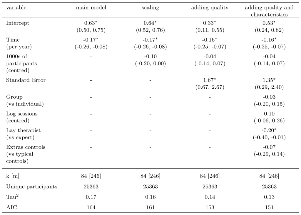
Note. All the effects presented above the first separation line are coefficients from the meta-analysis model. Their effects are in Hedge’s g (SD changes). The parentheses represent 95% confidence intervals. Statistical significance is represented such that * p < 0.05; ** p < 0.01; *** p < 0.001.
This suggests to us that, beyond this finding being non-significant, the effect of scaling can be controlled away with quality variables, more of which that we have not considered here might be included. While we think this latter -0.04 SDs per 1,000 value is a more accurate estimate of how psychotherapy’s effects may decline as an intervention scales, we do not think it is appropriate to extrapolate this figure (from admittedly limited modelling) to predict the effect of the charities as they operate at scale. Especially considering that while it is technically possible to extrapolate this figure to predict the effect of the charities as they operate at scale, this would mean a prediction far outside the data the model was fit on (~200,000 vs the largest sample in our study being ~7,000), which heavily undermines the validity of such an estimate.
This updates us towards thinking that the relationship between sample and effect size is largely moderated by study quality and observable study characteristics. DellaVigna and Linos (2022) is the only study we have found that attempts to explain how the effectiveness of an intervention (nudges to change behaviour in this case) is smaller (down to 24% the size of the original) at higher scales. However, they do not ascribe any of this to an actual decline in intervention effectiveness. They estimate this is around 70% attributable to publication bias, with most of the rest (they unfortunately do not provide a precise figure) attributable to differences in nudge types (i.e., observable intervention characteristics). This parallels our analysis above.
Vivalt (2020) do find evidence suggesting that larger trials tend to have smaller effects. In a meta-analysis of 635 RCTs of 20 development interventions, Vivalt finds a significant -0.01 SDs decrease in effect per 100,000 increase in sample size (with an intercept of 0.5 SDs) – which suggests very large interventions were included. If we take the Vivalt figures, then this would imply that the charities, due to scale, should have a lower effect of ~2 * -0.01 = -0.02 SDs. This is a very small effect, which implies a 1-(0.02/0.50) = 0.96 adjustment (4% discount) compared to their intercept of 0.50 and 1-(0.02/0.70) = 0.97 (3% discount) for the general effect of psychotherapy of ~0.7 SDs as measured in the literature (Cuijpers et al., 2018). Furthermore, it does not incorporate our concern that this may be overwhelmingly driven by study characteristics and study quality (see above) – which Vivalt (2020) did not control for.
Vivalt’s (2020) results imply that the difference between academic/NGO-implemented programmes and government-implemented programmes is -0.05 SDsIn Table 7 of Vivalt (2020), the difference between government-implemented and the private sector is -0.07 SDs and the difference between academic/NGO-implemented and the private sector is -0.02 SDs, which implies a difference between government-implemented and NGO-implemented of 0.07 - 0.02 = -0.05 SDs.. StrongMinds’s partners are government workers in 55% of cases. Using Vivalt’s estimates, this would imply a decrease of -0.05 * 55% = -0.03 SDs in effectiveness. When we apply this to ~0.7 SDs, this represents a 1-(0.03/0.70) = 0.96 adjustment (a 4% discount).
If we look at the charities themselves and how they are performing, we do not think they show strong losses in effectiveness due to scaling. If we look at the charity-related pre-post evidence, we find the charities to be effective (see Section 4.3). Looking at the pre-post results for StrongMinds over timeFriendship Bench do not report the pre-post results in the annual report in an easy way to extract., we do not see a strong decline in effectiveness as the charity has scaled up (see Table I3).
Table I3: StrongMinds’ pre-post scores over the years.
|
Year |
Total Clients Treated |
Pre-Post Change on PHQ-9 |
Naive Average Pre-Post Change |
|
2018 |
18,963 |
-13 points |
-13.00 |
|
2019 |
23,036 |
-13 points (SM-led), -12 points (peer-led) |
-12.50 |
|
2020 |
11,390 |
-13 points (SM-led), -12 points (peer-led) |
-12.50 |
|
2021 |
42,483 |
-13 points (SM-led), -13 points (peer-led), -12 points (partner-led) |
-12.70 |
|
2022 |
107,471 |
-11.7 points (SM-led), -12.4 points (peer-led), -11.3 points (government-led), -10.7 points (NGO partner-led) |
-11.50 |
|
2023 |
239,672 |
-13.9 points (SM-led), -9.7 points (NGO partner-led), -12.9 points (peer facilitators), -12 points (government partners) |
-12.10 |
We think it is also plausible that the charities have been maintaining the quality of the intervention by gaining experience and iterating on it over time. Finally, they also plausibly have positive externalities related to their scaling and collaboration with governments in the form of destigmatising mental health and influencing government policy towards more effective funding for mental healthcare.
Appendix J: Quality of evidence details
In this appendix we present the details of our evaluations of quality of evidence for different parts of our analysis. Our quality of evidence assessments are based on the GRADE criteria (Schünemann et al., 2013). Note that our criteria for evidence quality is stringent. See Section 2.6.1 for more explanation.
J1. General meta-analysis of psychotherapy
We assess the overall quality of evidence of the general causal evidence to be ‘moderate’ overall. The evidence base includes a large number of RCTs, with decently precisely estimated effects and limited risk of bias. However, there is some inconsistency in the effect sizes (measured as heterogeneity), and the studies are not directly related to the contexts of the charities. There is also substantial publication bias that — while adjusted for — may still bias the results. See detail below.
Study design: High quality
The sample includes RCTs, which are the best study design for determining causal effects, so the evidence is high quality for the study design criteria.
Risk of Bias: Some concern
To improve the average quality of the evidence we use, we remove studies that have high risk of bias (NB: we do not remove studies with ‘some concerns’ in order to maintain a sufficient sample size). After removing high RoB studies, 57% of those remaining are rated as some concern, and 43% are rated as low risk of bias. Because the majority of the studies are rated as ‘some concern’, we rate the quality of evidence on the RoB criteria as some concern.
Imprecision: No concern
This is a very large meta-analysis (k = 84) and sample size (N = 25,363). As shown in Section 4.1, the initial effect on recipients and the decay over time are significant. The total effect on the individual (i.e., not including spillovers and before validity adjustments) is 2.05 (95% CI: 1.16, 4.60) WELLBYs, which, for reference, is slightly more precisely estimated than the total effect in our analysis of cash transfers (McGuire et al., 2022b)We multiply the SD-years results 1.05 (95% CI: 0.21, 2.84) by the SD-years to WELLBY ratio we currently use which is 1:2. : 2.10 (95% CI: 0.42, 5.68) WELLBYs. Because these effects are measured with large samples and adequate precision to exclude 0 effect, we rate the quality of evidence on the imprecision criteria as no concern.
Inconsistency: Some concern
Heterogeneity is difficult to interpret (Kepes et al., 2023). As shown in Appendix C2, heterogeneity is substantial, and much higher than for our meta-analysis of cash transfers. However, it is unclear at which point the heterogeneity should start causing major concerns. The fact that we can account for some of the variability with moderators is reassuring that we are not clueless as to how psychotherapy in LMICs performs. Because there is still heterogeneity we are unable to explain, and that it is higher than for cash transfers, we rate the quality of evidence on the inconsistency criteria as some concern.
Indirectness: Some concern
The meta-analysis includes psychotherapy interventions in LMICs, where most of the sample are participants with depression, anxiety, or other forms of psychological distress. While these general characteristics overlap significantly with those of StrongMinds and Friendship Bench, the more specific details of the context and implementation of the interventions differ in a variety of ways, so we rate the quality of evidence on the indirectness criteria as some concerns, even after adjusting for as many characteristics as we could (see Section 5.2). For Friendship Bench, we have some additional uncertainty about the low dosage, but our alternative modelling (Section 5.2.3 and Appendix H) suggests that more severe adjustments would have limited impact on the cost-effectiveness, so we maintain the rating as some concern.
Publication bias: Some concern
Diagnostic tests suggest a significant amount of publication bias. Based on estimates from our panel of methods, we apply an adjustment of 0.69 (31% discount) to the effect. While this adjustment represents our best guess of the effect after controlling for publication bias, publication bias adjustment methods are limited, so we have some uncertainty about the size of the adjustment. Therefore, we rate the quality of evidence on the publication bias criteria as some concern.
J2. Friendship Bench RCTs
We assess the overall quality of evidence of the Friendship Bench RCT evidence to be ‘low to moderate’. While there are only a small number of studies (k = 4), the sample size is decent, the studies are mostly relevant, the imprecision and inconsistency are moderate, and we have relatively little concern about publication bias. The biggest concern is about risk of bias and the low dosage which affects indirectness. See detail below.
Study design: High quality
The sample includes RCTs, which are the best study design for determining causal effects, so the evidence is high quality for the study design criteria.
Risk of Bias: Major concerns
In our risk of bias evaluation, we evaluated Haas et al. (2023), and Bengtson et al. (2023), to each be ‘some concerns’. Simms et al. (2022) and Chibanda et al. (2016) were ‘high’ risk of bias. As we discussed in Section 3.2.1, we do not actually think that this rating warrants removing these studies, especially not Chibanda et al.
Additionally, Dr Dixon Chibanda, the founder of Friendship Bench, is an author on three of the publications. While we do not have any specific reason to believe this has introduced bias in these studies, we think the risk of bias is generally higher when authors are not completely independent from the intervention being studied.
Overall, we rate the quality of evidence on the RoB criteria as major concerns.
Imprecision: Some concern
This is a small meta-analysis of 4 RCTs (N = 2,011). The initial effect on recipients is significant (0.53, 95% CI: 0.04, 1.01) but the decay over time is not significant (-0.16, 95% CI: -0.49, 0.17). The total effect on the individual (i.e., not including spillovers and before validity adjustments) is 1.71 (95% CI: 0.04, 25.83) WELLBYs. Because of the mix between a significant intercept and a non-significant decay over time, we rate the quality of evidence on the imprecision criteria as some concern.
Inconsistency: Some concern
Surprisingly the heterogeneity of the Friendship Bench RCTs is very similar to the general psychotherapy analysis (see Appendix C2), despite there being a lot fewer studies and all of these being about the same programme. The low number of studies means that we cannot, and have not, added many moderators to attempt to explain away the heterogeneity. Because it is similar to the general evidence, we also assess it as some concern.
Indirectness: Some concern
The population and context of the studies are generally very similar to that of Friendship Bench as it operates, with a few differences. Like Friendship Bench, three of the trials are with adults (while one is with adolescents), three trials are set in Zimbabwe (one is in Malawi), three of the trials provide in-person individual psychotherapy delivered by a lay counsellor (one is via phone). Unlike Friendship Bench, three trials exclusively involved participants with HIV, and the studies reported attendances closer to 5/6 sessions of psychotherapy (Friendship Bench participants attended an average of 1.12 sessions). The studies are overwhelmingly similar to the context of Friendship Bench, but because of the important uncertainty about dosage (see Section 5.2.3 and Appendix H), we rate the quality of evidence on the indirectness criteria as some concern.
Publication bias: Some concern
Three out of the four Friendship Bench RCTs are pre-registered and seem to have, overall, followed their protocols. We applied an adjusted publication bias adjustment. Overall, we think this is only of some concern.
J3. Friendship Bench pre-post
We assess the overall quality of evidence of the Friendship Bench pre-post evidence to be ‘very low’. The primary reason is that we do not have a true control group, and our pseudo-synthetic controls method provides limited information. There is also the potential for substantial risks of bias. See detail below.
Study design: Low quality
The Friendship Bench M&E data consists of pre-post scores from participants in their programme. Because there is not a comparable control group, this type of study design is considered low quality for its lack of comparator and causal explaining power. However, we estimate the effects using a pseudo-synthetic control approach. While this offers an improvement over having no control group, the accuracy of the results is still limited (see Appendix K for more detail). Therefore we rate the quality of evidence on the study design criteria as low. Based on the GRADE process, this means that the overall evidence quality should be considered low as a starting point.
Risk of Bias: Major concerns
Because we do not have a published report about the M&E data, we cannot formally assess risk of bias. That being said, we generally assume that M&E data will have high risk of bias. Pre-post data from a charity – even if it uses an external agency to collect the data – will have some risk of bias. We think that there is some potential for some (likely unintended) bias, such as whether samples are from participants who experienced a greater effect, some surveyors might induce bias, and there could be some selection in the data when it came to the analysis. We adjust for this with a 0.51 replicability adjustment factor derived from the literature (which is more severe than publication bias) and with a 0.85 adjustment for response bias. Overall, we rate the risk of bias as major concerns.
Imprecision: Major concerns
The initial effect on the recipient is estimated to be 0.12 (95% CI: 0.04, 0.19) SDs, based on a sample of 3,423 Friendship Bench clients. The confidence interval does not include 0, and is fairly narrow. However, we are uncertain about our pseudo-synthetic control method. The duration is taken from the prior. The total effect on the recipient (i.e., not including spillovers and before validity adjustments) is 0.41 (95% CI: 0.14, 1.00) WELLBYs. Taken together, we rate the quality of evidence on the imprecision criteria as major concerns.
Inconsistency: Major concerns
We are not able to assess inconsistency directly. Thus, we rate the quality of evidence on the inconsistency criteria as major concerns. However, we can compare this study against the general evidence and the RCT data. The effect of this study is smaller than the other data sources.
Indirectness: No concern
This data comes directly from Friendship Bench as it implements its programme, so we do not have any concern about indirectness.
Publication bias: Not applicable.
Publication bias does not apply to charity M&E data, since it does not go through the academic publishing process.
J4. StrongMinds RCTs
We assess the overall quality of evidence of the StrongMinds RCT evidence to be ‘low’. There is only one RCT (Baird et al., 2024), which means we are unable to assess inconsistency. While it has a decent sample size and was pre-registered so we are less concerned about publication bias, its relevance to StrongMinds’ current program is potentially limited. See detail below.
Study design: High quality
The sample includes one RCT, which is the best study design for determining causal effects, so the evidence is high quality for the study design criteria.
Risk of Bias: Some concerns
This study was very recently published as a working paper (i.e., it has not been through the academic publication process and peer review, which means the results are more susceptible to changing). Our risk of bias evaluation of Baird et al. (2024) is that it is ‘some concerns’, notably because of issues of complianceIn our risk of bias assessment, we evaluated Baird et al. (2024) as ‘some concerns’ because of its low levels of compliance (44% of participants failed to attend any sessions). Baird et al. explore the effect of compliance using a LATE analysis (see Section 5.2.4), but the ROB criteria still considers this to lead to ‘some concerns’. On the other subdomains we evaluated Baird et al. to be ‘low’ risk of bias..
Imprecision: Some concerns
There is only one RCT that we consider being charity-related evidence for StrongMinds (Baird et al., 2024), with N = 1,896. This is a decent sample size, but only a single study. The initial effect on recipients is significant (0.10, 95% CI: 0.01, 0.19) but the decay over time is not significant (-0.07, 95% CI: -0.13, 0.00). The total effect on the recipient (i.e., not including spillovers and before validity adjustments) is 0.15 (95% CI: 0.00, 1.42) WELLBYs. We rate the quality of evidence on the imprecision criteria as some concerns. Although we are concerned by there being only one study, we also consider this under our rating of inconsistency below.
Inconsistency: Major concerns
Because there is only one study in this evidence base, we are not able to assess inconsistency directly. However, we can compare this study against the general evidence and the M&E data. The effect of this study is substantially different from the other data sources. For these reasons, we rate the quality of evidence on the inconsistency criteria as major concerns. Furthermore, the Friendship Bench RCTs have levels of heterogeneity close to those of the general psychotherapy analysis, so we would be surprised not to find a similar pattern if we had more RCTs for StrongMinds.
Indirectness: Major concerns
While this study provides evidence of an implementation of StrongMinds’ programme, there are reasons to believe its representativeness of StrongMinds in general is limited. See Section 7.3 and Appendix L for extensive discussion. We adjust our estimates for the higher number of sessions, issues with non-compliance, and focus on teenagers (vs adults), but we do not think this fully adjusts for these deviations from how StrongMinds implements its programme. We think Baird et al. (2024) captures some aspects of StrongMinds’ impact, but it definitely has key limitations, so, we rate the quality of evidence on the indirectness criteria as major concerns.
Publication bias: No concerns
This study was pre-registered, and it is the only RCT we are aware of studying the impact of StrongMinds directly. Therefore, we have no concerns about publication bias.
J5. StrongMinds pre-post
We assess the overall quality of evidence of the StrongMinds M&E pre-post evidence to be ‘very low’. The primary reason is that we do not have a true control group, and our pseudo-synthetic controls provide limited information. There is also the potential for substantial risks of bias. See the details below.
Study design: Low quality
The StrongMinds M&E data consists of pre-post scores from participants in their programme. Because there is not a comparable control group, this type of study design is considered low quality for its lack of comparator and causal explaining power. However, we estimate the effects using a pseudo-synthetic control approach. While this offers an improvement over having no control group, the accuracy of the results are still limited (see Appendix K for more detail). Therefore we rate the quality of evidence on the study design criteria as low. Based on the GRADE process, this means that the overall evidence quality should be considered low as a starting point.
Risk of Bias: Major concerns
Because we do not have a published report about the M&E data, we cannot formally assess risk of bias. However, from our work with StrongMinds, we get the impression that their M&E data is high quality, and StrongMinds have mentioned that their data is validated by an external agency (see 2023 Q4 report). That being said, pre-post data from a charity - even if it uses an external agency to collect the data - will have some risk of bias. We think that there is some potential for some (likely unintended) bias, such as whether samples are from participants who experienced a greater effect, some surveyors might induce bias, and there could be some selection in the data when it came to the analysis. We adjust for this with a 0.51 replicability adjustment factor derived from the literature (which is more severe than publication bias) and with a 0.85 adjustment for response bias. Overall, we rate the risk of bias as major concerns.
Imprecision: Major concerns
The initial effect on the recipient is estimated to be 0.79 (95% CI: 0.74, 0.84) SDs, based on 218,045 StrongMinds clients. The confidence interval does not include 0, and is fairly narrow. However, we are uncertain about our pseudo-synthetic control method. The duration is taken from the prior. The total effect on the recipient (i.e., not including spillovers and before validity adjustments) is 2.75 (95% CI: 1.71, 5.91) WELLBYs. Taken together, we rate the quality of evidence on the imprecision criteria as major concerns.
Inconsistency: Major concerns
As above with the StrongMinds RCT data, we are not able to assess inconsistency directly, so we rate the quality of evidence on the inconsistency criteria as major concerns. Comparing this study against the general evidence and the RCT data, the effect is not substantially different (albeit a bit higher) from the other data sources.
Indirectness: No concerns
This data comes directly from StrongMinds as it implements its programme, so we do not have any concern about indirectness.
Publication bias: Not applicable
Publication bias does not apply to charity M&E data, since it does not go through the academic publishing process.
J6. Spillovers
We assess the overall quality of evidence of the spillover evidence to be ‘very low’. This is primarily due to there being so few studies, especially RCTs, available on this topic. See the details below.
Study design: Moderate quality
This evidence base consists of 4 RCTs + 5 observational studies and 2 natural experimentsNote that the number of studies itself is a factor for the ‘imprecision’ criteria.. Our estimate of the effect averages two analyses: one using the RCT evidence and one using the RCT evidence and some the non-RCT evidence split across pathways. Given the mix of study designs we rely on, we rate the quality of evidence on the study design criteria as moderate.
Risk of Bias: Major concern
Only two of the RCTs (Barker et al. and Bryant et al.) have been assessed for risk of bias, and they were both rated as ‘some concerns’. The other studies have not been assessed. Given this uncertainty, we rate the quality of evidence on the RoB criteria as major concerns.
Imprecision: Major concerns
There are very few studies determining such an important part of our analysis. Getting a confidence interval for a ratio is not straightforward, so we have to use Monte Carlo simulations. However, we analyse spillovers in two ways. The pathways analysis does not lend itself easily to analysing uncertainty, but considering it is a duct-taping of many different small sources of data, the uncertainty should be considered high. The meta-analytic analysis lends itself a bit more but suggests an unbelievable range of -107% to 164%. Instead, we conclude that the uncertainty is really high and that more research in this area is necessary. For the purpose of using uncertainty in our analysis, we give the spillover ratio a beta distribution with a 95% CI of 0% to 50%, representing that we are very uncertain but that we think that the results could not be above 100% or below 0%. Because of the wide range of possible values, we rate the quality of evidence on the imprecision criteria as major concerns.
Inconsistency: Major concerns
The meta-analytical analysis (12%) and pathway-analysis (21%) suggest different spillover ratios, and the individual studies imply an even wider range of potential ratios. We take the average of the two figures. But, given the differences between the figures, we rate the quality of evidence on the inconsistency criteria as major concerns.
Indirectness: Major concerns
The studies take place in different contexts to that of StrongMinds and Friendship Bench, and each study looks at the effects on different household member pairs. It is unclear how well these effects capture the spillover effects of the charities, so we rate the quality of evidence on the indirectness criteria as a major concerns.
Publication bias: No concern
We are unsure about the publication bias, but think it is probably low since almost all results were not reported with the intent of being used to estimate household spillovers. Because this was not the central effect of these studies, it is less likely that these effects determined whether the studies were published. Although, there could still be some indirect publication bias if (a) the studies were published based on the significance of the wellbeing effects and (b) the wellbeing effects were related to the spillover effects.
Appendix K: Using M&E pre-post data
We add M&E pre-post as a source for the effect of charities psychotherapy programmes in practice. We have pre-post data that the charities collect during routine M&E. This data could be the most relevant data available about the charities, for these are the effects of the latest work from the charity. Hence, it could be more relevant than general RCTs in LMICs (i.e., they are not about the charity directly) and RCTs of the charities (i.e., they are not necessarily exactly how the intervention is currently implemented).
However, pre-post estimates (i.e., within-person effects) do not have a control group to compare the results to (i.e., do not have between-person effects), which means results will be inflated compared to RCT between-effects and, additionally, would lack causal explanatory power (Morris & DeShon, 2002; Cuijpers et al., 2016). Omitting a control group can confound the results; notably, participants’ levels of depression might reduce – to some extent – even without psychotherapy (i.e., spontaneous remission; Cuijpers et al., 2014), making the reduction in the treatment group (the within-effect) an overestimate if not compared to a control group (to calculate the between-effect). In order to make pre-post results (i.e., within-effects) more comparable with RCT results (i.e., between-effects) we need to adjust for this overestimation.
Ideally, we would use a synthetic control groups methodology. To do so, we would have to find individuals in the same context as the charities, who reported results on the same scales as the charities, who we can match on important characteristics to the clients of the charities (e.g., initial levels of mental distress, demographics, socio-economics, etc.), and who did not receive the intervention. We could not find data that would fit these demands. However, we do have data about control groups in our general RCTs of psychotherapy in LMICs.
So, we use a simpler, ‘pseudo-synthetic’ control approach where we take RCTs from our general meta-analysis which use the same scales as the charities. We then take a weighted average of their control groups to form our pseudo-synthetic control group for the pre-post data. In other words, we use the data from the control groups from other contexts (of varying similarity, at the very least in LMICs and using the same scales) to act as our control group for assessing the monitoring and evaluation data. This is not ideal, but it adjusts for issues of using pre-post data better than not using a control group. Thereby, this unlocks what could be the most relevant data.
We are extremely uncertain about our methodology here, and acknowledge that it is not a standard process. Nevertheless, we give little weight to the pre-post data (less than 17%; see Section 7) and we check how robust data sources are to different data sources (see Section 9.3).
K1. The method
In Version 3.5 of this report (McGuire et al., 2024) we used 6 different possible methods because we were uncertain which was the best method to use. We now use one method, which is more statistically valid than the othersWe received feedback on our methods from Statistics Without Borders, who noted disadvantages with the alternative approaches and suggested the current approach. .
Our aim is to get as accurate an effect size for the pre-post M&E data as we can. We can calculate an effect size from pre-post data (Lakens, 2013):
$$ d_{\text{pre-post}} \;=\; \frac{M_{\text{pre}} -
M_{\text{post}}}{\text{mean}(SD_{\text{pre}},\, SD_{\text{post}})} $$
However, the core difference here is that the numerator (the “pre-post mean difference”, hereafter the “within-effect”) is based on comparing the mean of the group before and after treatment. The mean difference for effect sizes we use in a meta-analysis (hereafter the “between-effect”) is comparing the treatment and control group after treatment (Lakens, 2013)Another difference is the exact denominator in standard deviations.:
$$ d_{\text{RCT}} \;=\; \frac{M_{\text{control}} -
M_{\text{treatment}}}{\text{pool}(SD_{\text{control}},\, SD_{\text{treatment}})} $$
The aim, therefore, is to adjust the within-effect as if it had a comparative control group in order to produce a “synthetic between-effect”; therefore, removing potential overestimation that would have occurred if we relied only on the within-effect.
Therefore, what we want to do is take the \(M_{\text{treatment}}\) from the M&E data (the post mean) and find an \(M_{\text{control}}\) that we can use. For each charity pre-post data we select studies from our general meta-analysis of psychotherapy in LMICs which use the same outcomes as the charities (PHQ-9 for StrongMinds and SSQ-14 for Friendship Bench). We then average the \(M_{\text{control}}\) of each study according to their sample size to provide an \(M_{\text{control}}\) for the calculation of the effect size of the pre-post data.
K2. Results
We present the results for both charities. Remember that these results are on affective mental health scales where lower results are better (i.e., more wellbeing). Hence, small post treatment means for the treatment group are a good sign and large reductions in symptoms are a good sign.
K2.1 Friendship Bench
We use 2023 pre-post data from 3,326 Friendship Bench clients (see Section 3.3.1 for more detail). There is an average reduction in symptoms of -4.13 points on the SSQ-14 (a 14 point general mental distress scale, so higher scores represent worse wellbeing). The post-treatment mean is 5.23 (SD = 3.06) points.
The reference RCTs are studies which also measure outcomes on the SSQ-14. This happens to be three Friendship Bench studies (Chibanda et al., Simms et al., and Haas et al.). This means these are likely representative reference studies. However, this also means this analysis is heavily double dipping with information from the Friendship Bench RCTs. We use the earliest follow-up possible for each study so that it is as close to the timing of the M&E pre-post as possible. See Table K1 at the end for more detail.
The sample size weighted post-treatment control mean was 5.62 (SD = 4.06)The SD was pooledacross the studies.. This leads to a mean difference of 5.62 - 5.23 = 0.39 points. The pooled SD is 3.30. The effect size for this data, with this pseudo-synthetic-control method, is g = 0.12 SDs.
This is potentially conservative considering the reference RCTs all were ‘enhanced usual care’ control groups rather than ‘nothing’ as is typically available to people in Zimbabwe.
K2.2 StrongMinds
We use pre-post data from StrongMinds. In 2023, they had post treatment scores for 218,045 clients in Uganda and Zambia. This is almost all of their clients. The average reduction in symptoms of -13.04 points on the PHQ-9 (27 points depression scale, so higher scores represent worse wellbeing) – a very large reduction. See Section 3.3.2 for more detail. The post-treatment mean is 2.49 (SD = 1.94) points.
To build our comparison group for StrongMinds, we used the 12 reference RCTs from our general meta-analysis that measure changes in the PHQ-9. See Table K2 at the end for more detail. Note that none of these studies are a direct study of a StrongMinds intervention. Also note that Haas et al., because they have results both in the PHQ-9 and the SSQ-14, is included here as well as in the reference RCTs for Friendship Bench.
The effect size for this data, with this pseudo-synthetic-control method, is g = 0.79 SDs. We explain the elements that go into this calculation because there were multiple choices possible and we used the most conservative.
The sample size weighted post-treatment control mean was 7.10 (SD = 5.83)The SD was pooledacross the studies.. This leads to a mean difference of 7.10 - 2.49 = 4.61. Note that the choice of this control mean is conservative because other options (the mean from Baird et al., the mean from the controlled but not randomised trial of StrongMinds adults, and another technical option for calculating the post-treatment control meanThis was suggested to us by Statistics Without Borders. Using the reference RCTs, we use a weighted linear model to predict the post-treatment control mean based on the baseline control mean. This suggest that a post-treatment control mean on the PHQ-9 is equal to 2.88 + b* 0.37 where bis the baseline level. StrongMinds’s M&E data finds a baseline level of 15.53, which would predict a post-treatment control mean of 8.63.) were all higher (i.e., suggested the control group was worse off, so less spontaneous remission or regression to the mean occurred). See Table K3 for more detail.
The second important part of the calculation of an effect size is the SD pooled. This is a sample size weighted average of the SD of the control and treatment group SDs. The SD for the StrongMinds’s M&E is 1.94, which is much smaller than the 5.83 SD from the synthetic control group. With a sample size of 218,045, the SD from StrongMinds’s M&E would dominate the pooled SD and lead to a g = 2.32. The large sample size suggests that StrongMinds's M&E SD is a more accurate estimate of the population SD according to the central limit theorem. However, when there is such an important difference between the two standard deviations it is typical to use the SD of the control group (i.e., Glass’s delta; Lakens, 2013). Therefore, we use the larger SD as the SD pooled which leads to a much more conservative estimate.
Note that Table K3 is also useful for exploring why the results from the StrongMinds’s M&E are so different from Baird et al.’s trial. There are three important elements: the starting baseline level, the post-treatment treatment group mean (i.e., how potent the intervention was), and the post-treatment control group mean (i.e., how much of the effect can be explained away by things like natural recovery/spontaneous remission/regression to the mean/etc.). Here are a few patterns we observe:
- The StrongMinds M&E data and the controlled (but not randomised) trial on StrongMinds adults (Peterson et al., 2024) have very similar pre and post treatment group results.
- It is difficult to untangle, but the pre-post changes (-13.04 for StrongMinds; -5.27 for Baird et al.) suggest that the programme in Baird et al. was less effective (see Appendix K2.2 for more detail), reinforcing the idea that the programme in Baird et al. might simply be a failed implementation because of its contextWe acknowledge that an alternative could be that the M&E results are inflated, but we think that the issues with Baird et al. are more likely.. After treatment, the treatment group in Baird et al. had much higher levels of depression (7.90 points) than clients in StrongMinds’ M&E (2.49 points)StrongMinds’s M&E is on the PHQ-9 scale (a 27 points depression scale), so higher scores are worse. Baird et al. uses the PHQ-8, which is the PHQ-9 without the question about suicidal ideation, making it a 24 point scale (i.e., when linearly transformed, its results are higher). In the case of the post-treatment treatment group mean it would be 7.90 * 27/24 = 8.89..
Table K1: Characteristics of the reference RCTs for Friendship Bench.

Table K2: Characteristics of the reference RCTs for StrongMinds.

Table K3: Pre-post results for different data sources on the PHQ-9.
|
Source |
Baseline (pre) mean for the treatment group |
Endline (post) mean for the treatment group |
Treatment group pre-post |
Endline (post) mean for the control group |
Mean difference |
|
StrongMinds M&E on the PHQ-9 |
15.53 |
2.49 |
-13.04 |
Not included, because it is just a pre-post, we used the mean from reference RCTs because it was the most conservative: 7.10 |
(after using our pseudo-synthetic-control method:) -4.61 |
|
Weighted average from reference RCTs who use the PHQ-9 scale |
11.82 |
5.69 |
-6.13 |
7.10 |
-1.41 |
|
Baird et al. (2024) on the PHQ-8 |
13.17 (linearly transformed: 14.82) |
7.90 (linearly transformed: 8.89) |
-5.27 |
8.20 (linearly transformed: 9.23) |
-0.30 |
|
StrongMinds’ controlled (but not randomised) trial (Peterson et al., 2024) on the PHQ-9 |
15.58 |
2.86 |
-12.72 |
9.07 |
-6.21 |
Note. The PHQ-9 scale is a 27 point depression scare, so higher scores are worse. Baird et al. (2024) uses the PHQ-8, which is the PHQ-9 without the question about suicidal ideation, making it a 24 point scale (i.e., when linearly transformed, its results are higher).
Appendix L: Weighting Methods
In Section 7 we discussed our weighting methodology and the weights we attributed. Here, we discuss some methodological details in more depth (Appendix L1), compare weights across the two charities (Appendix L2), and discuss the limited relevance of the Baird et al. (2024) study to StrongMinds (Appendix L3). If readers disagree with our weighting system they can form their own view of what would be the resulting cost-effectiveness of the charities according to the weightings in Section 7.4.
L1. More details about weighting methodology
L1.1 Bayesian methodology
To calculate the quantitative weights based on statistical uncertainty we use Bayesian updating. According to Bayes’ rule, we can integrate two continuous probability distributions (often called the prior and the likelihood/data), to produce a new distribution (the posterior). From this process we can determine how much weight each initial distribution had in determining the posterior; what we refer to as the Bayesian-informed weight. In our case, the two distributions we are combining are the effect (after adjustments)We use the total effect on the individual (after adjustments), but this would not change if we used the overall effect on the household because the household spillovers we apply are the same for each evidence source. for the general meta-analysis of psychotherapy in LMICs and the charity-related RCTs. These distributions were determined using Monte Carlo simulationsBecause the total effect is an integral over time, it is not easy to derive a confidence interval and a distribution. Instead, we use Monte Carlo simulations that allow us to approximate the distribution. We limit the simulations so that each simulation will produce an integral of an effect decaying to zero (see Section 2). We prevent the simulations from generating negative initial effects (which seems plausible considering all the initial effects across the sources of evidence are statistically different from zero) and prevent the trajectory over time from generating cases of growing benefits over time (rather than decay). Note that one has to make decisions about how to run the integral and we believe this is a plausible one. If we weaken these constraints, the Bayesian updating process is almost unaffected (it would, mainly, give less weight to Baird et al., the source of evidence closest to 0, and thereby, the one most benefiting in weight from increased certainty due to the constraints)..
While an analytical solution exists when both distributions are simple (e.g., two normal distributions), our total recipient effects show positive skew (because they are the result of integrating the initial effect over time), making an analytical solution impractical. Instead, we employ grid approximation (McElreath, 2020; Johnson et al., 2021), an effective and common Bayesian technique given our single-parameter model that can easily incorporate non-standard distribution shapes. We describe it below.
In this approach, we partition a probability space for total recipient effects, ranging from -1 to ~200 WELLBYsThe exact range of the grid doesn’t matter as long as it covers plausible space across which the prior and new data distributions are specified. The range for StrongMinds was -1 to 28 WELLBYs, and -1 to 183 WELLBYs for Friendship Bench. We selected this range based on the 99th percentile of the prior and data distributions of total effect on the recipient for each respective charity., into 100,000 discrete outcomes (i.e., the grid). For each discrete point, we determine the probability density from both the prior and the data. Bayes’ rule is then applied to produce the posterior probability density for each point. Specifically, we multiply the prior by the data for each point on the grid; this gives us the unnormalized posterior. We then normalise the posterior (i.e., divide by the sum of all such multiplications across the grid so that it sums to one). The posterior is subsequently approximated by randomly sampling 100,000 values from this normalised grid to estimate statistical measures like the mean and credible intervals for further analysis.
This method is conceptually similar to a Riemann sum, wherein a continuous function is approximated using discrete partitions. The greater the number of partitions, the more accurate our approximation becomes, akin to improving resolution (see Johnson et al.’s rainbow image illustration). Although this might sound complex, it is among the easiest Bayesian approximation methods to implement and is well-documented in Bayesian statistics textbooks (McElreath, 2020; Johnson et al., 2021).
If we had just two simple sources to combine (i.e., the general meta-analysis and the charity-related RCTs), we would just use the posterior and continue to the cost-effectiveness part of the analysis from there. This is what people would typically do with a Bayesian analysis. We do not do this for two reasons: (1) we want to derive weights so that we can then subjectively adjust them (see Section 7.1) and (2) we have a third evidence source – the M&E pre-post data – which we are uncertain about the methodology and, thereby, do not want to directly include formally in statistical weights.
The next step is to calculate the weight that each distribution provides. An easy approach which be to calculate the weight according to the means of each distribution:
$$ Z \;=\; Xw + Yv $$
$$ w \;=\; (Z - Y) / (X - Y) $$
This method works well when the distributions are normal (symmetrical and not skewed). However, when dealing with skewed distributions, this approach may break down. Skewness can cause the posterior mean to fall outside the range of the prior and likelihood means (i.e., lower or higher than both means), which would make this calculation inaccurate. Instead, we use the grid to calculate the weight where we give each point on the grid a weight based on the value of the probability density for each distribution – which we then sum over to have the weight for each distribution:
Instead, we use the grid approximation to calculate the weight for each distribution. At each point on the grid, we assign a weight based on the probability density values for the prior and likelihood at that point using the formula belowIf the denominator of this calculation equals zero for a point on the grid, we give each distribution a 50% weight because we cannot divide by zero.. We then sum over to have the weights at each point for each distribution to get the weight for the prior and the weight for the likelihood.
$$ w_i \;=\; X_i / (X_i + Y_i) $$
See Figures L1 and L2 for an illustration of this grid approximation process with the total effect on the recipient (after adjustments) for the general meta-analysis of psychotherapy in LMICs and the charity-related RCTs. One can see that the probability density of the distributions for Friendship Bench share a lot more of the same space.
Figure L1: Grid approximation for Friendship Bench.
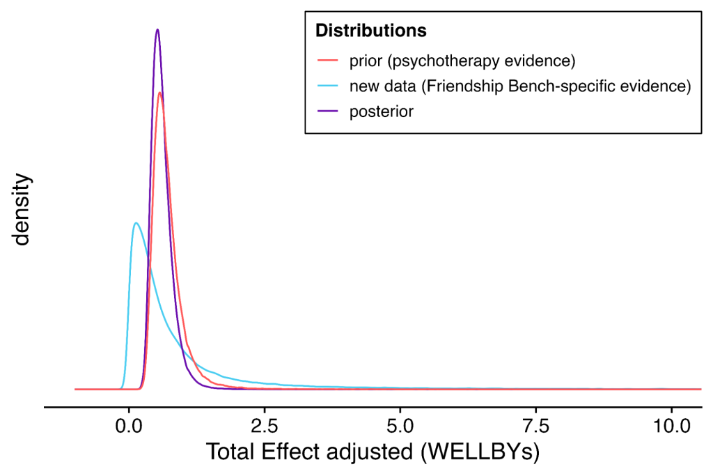
Figure L2: Grid approximation for StrongMinds.
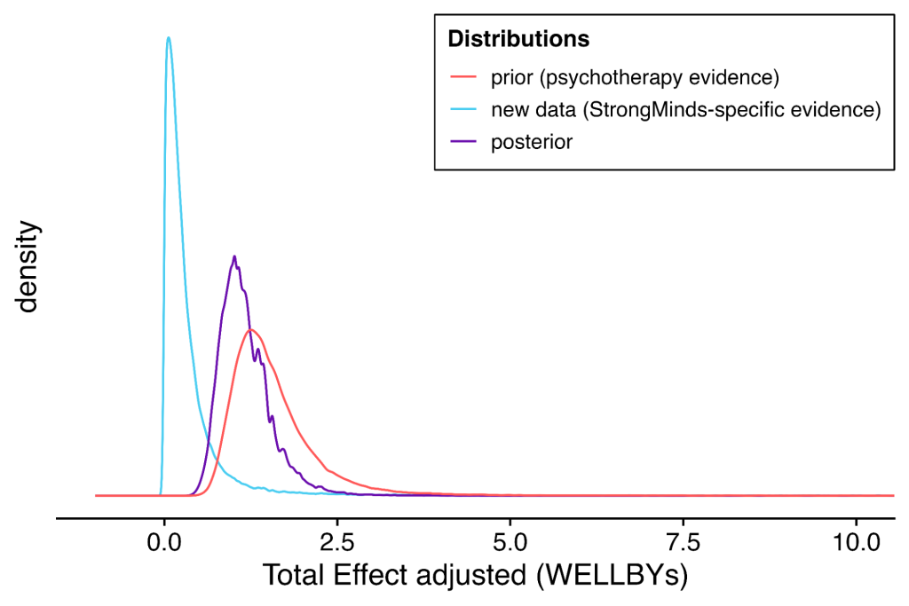
We discuss alternative modelling methods and considerations when we compare the weights of the different charities (see Appendix L2) and we discuss why we do not use uncertainty from percentile intervals for weighting below.
L1.2 Why not prediction intervals
It has been suggested to us that concerns about heterogeneity and generalisability could be integrated into quantitative weights by combining the τ2 with the SE of the meta-analysis in determining the uncertainty that goes into our Bayesian weights, akin to using the prediction interval (PI) rather than the confidence interval (CI) representations of uncertainty. In essence, a confidence interval indicates the range within which we think a ‘true’ value lies (i.e., the average, the expected value), while a prediction interval estimates the range within which a single future observation is likely to occur, which involves a greater level of uncertainty. However, to the best of our knowledge, using PIs to quantitatively include heterogeneity in weights lacks precedent (namely, we could not find any guidelines or practical academic discussion) and presents both conceptual and practical limitations, so we do not use it. Conceptually, we care about the expected value of the charities. Practically, it seems that forcing the uncertainty from the PIs into the Bayesian modelling is not a common method, and we might not even be able to calculate the PIs for every data source. We present the technical details for keen readers below.
Conceptually, CIs are about the uncertainty around the expected value (i.e., the average effect), whereas PIs are about predicting where the next observation (in the context of a meta-analysis, the next effect size) might fall. We are interested in the expected value of the different charities, not the next observation. Charities should not be seen as single observations but rather as entities with multiple studies estimating their effect. Hence, we should use the CI. The fact that our general evidence is about the expected value of psychotherapy in LMICs in general, and not the charities themselves, does not mean that the charities are individual observations within this literature. In other words, just because a source of data lacks perfect relevance does not mean that we treat our target as an observation within that data source. There are already multiple effect sizes from multiple studies for the different charities. Instead, we use the expected value of psychotherapy in LMICs as a prior for the expected value of the charities specifically, and then add our concerns about relevance of the data sources on top of this.
Practically, we have seen no precedent for using PIs as the uncertainty that determines the Bayesian-informed weights, nor is it even commonly doable in Bayesian software. Bayesian models update the average (g) and the heterogeneity (τ2) estimates based on the provided data, without merging them in the manner suggested by using the PI as the measure of uncertainty. To our understanding, the only practical way we would have of using the uncertainty as suggested by the PI is to provide the distribution it suggests to a simple method like Grid Approximation, ‘tricking’ it into thinking this is the uncertainty (to wit, we would be unable to perform this with rstan, a pillar of Bayesian software, for example). Again, this would be using the distribution which predicts the next observations rather than – as we conceptually argue above – the estimate of the expected value.
In our brief look at the literature on Bayesian Data Fusion (Koks & Challa, 2005) – which is one of the closest methods we have found to our weighting problem – we did not see mentions of using heterogeneity or PIs in such a way to influence the uncertainty and weighting in the Bayesian process.
Finally, this method is dependent on us being able to get accurate estimates of heterogeneity for each data source. There is only one StrongMinds-relevant RCT (Baird et al., 2024), thereby, there is no meta-analysis level heterogeneity. This would give that RCT a lot of weight but this seems misguided because there are four FriendshipBench RCTs and they have levels of heterogeneity that are very close to that of the general evidence, suggesting both that this method would not affect the Bayesian weighting very much and that with more StrongMinds RCTs we could find much higher estimates of heterogeneity.
While we think inconsistency can play a role in our weightings, we do not think this is the appropriate method. Instead, we use this information in our subjective weights based on principles of generalisability. We explain our qualitative criteria for our subjective weights next.
L1.3 The GRADE criteria and checklist
GRADE’s six criteria capture two broad categories of uncertainty.
First is the uncertainty related to a study’s quality (or internal validity). By quality, we roughly mean the degree to which replications would find similar effect sizes.
Second is the uncertainty related to its generalizability (or external validity). By generalizability, we mean the degree to which the effects of an evidence type would predict effects in a different context. For instance, suppose we have a study looking at the causal effect of psychotherapy, but it is carried out in the US in one-to-one sessions. How relevant is this data to our task of estimating the effects of StrongMinds intervention carried out in Sub-Saharan Africa (SSA) countries in group sessions? Having a sense of how generalisable evidence is to the charity, is crucial to our confidence in using it to predict the effects of the charity.
We discuss these factors in more depth below.
Quality factors
- Study design. We think we should put more weight on study designs with better causal identification strategies (RCTs rather than non-RCTs). This implies less weight for pre-post data because this data is lower down the causal hierarchy.
- Risk of Bias (RoB). RoB refers to limitations to the study design or implementation that might bias its estimated effects. We assessed RoB and removed studies with ‘high’ risk of bias, in part adjusting for this criteria. We think we should weigh evidence with lower (vs. higher) risk of bias more. Examples of issues that make risk of bias higher in RCTs:
- Participants are aware of the research question and the experimental conditions.
- Researchers are not blind to the condition participants are assigned to, or they have the ability to influence outcomes.
- There is sizable attrition (i.e., participants dropping out over the course of the study).
- There is sizable missing outcome data (i.e., missing data).
- Publication bias. Publication bias is a systematic bias in the publication of research findings that occurs when the outcome of a study influences whether or not it is published. We place more weight on evidence that is less likely to suffer from publication bias.
- Imprecision. Imprecision refers to how precisely effects are estimated; namely, statistical uncertainty. This depends on how many studies and participants are included. We can be more confident in a data source if it is more precisely estimated (e.g., more studies, larger samples). This criteria is the one already captured by our Bayesian-informed weighting because it will give more weight to the more precise sources.
Generalizability factors
- Inconsistency (heterogeneity). Inconsistency (or heterogeneity) refers to the variability between effect sizes (or studies more generally).
Unexplained heterogeneity suggests that there are moderating factors of the studies or the intervention itself that are not being captured. For example, in our psychotherapy meta-analysis, we find that moderating for the expertise of the deliverer reduces heterogeneity. High heterogeneity suggests that an intervention is not fully understood (Linden & Hönekopp, 2021).
Conversely, consistent results suggest that the effect is replicable (e.g., not a fluke finding) and robust (e.g., it does not depend on specific circumstances). High inconsistency between findings intuitively means low generalisability.
In a meta-analysis, heterogeneity is quantified as τ2 and presented along other indicators built on τ2 (I2, R2, and PI). Interpretation of these measures is not straightforward, making it difficult to determine if heterogeneity is ‘high’ or not (Harrer et al., 2021; Borenstein et al., 2022; Kepes et al., 2023; see Appendix C2 for more detail). One either has to compare between interventions or resort to vague guidelines (which is much less recommended). There is no clear, citable precedent of how to quantify weights for different sources based on heterogeneity; therefore, we looked at different indicators of heterogeneity across the sources to subjectively adjust weights.
- Indirectness (relevance). Indirectness refers to the relevance of the evidence to the real world context of the charity. Examples of characteristics that often differ between sources of evidence and the charity include: population demographics, expertise of deliverer, number and length of sessions, group or individual delivery format. In an ideal world, we are able to model any differences due to these factors, but in practice our quantitative models can only capture what we can observe, and when some features differ between less and more relevant pieces of evidence, it may represent the tip of the iceberg of factors that differ.
L2. Alternatives and comparing weights across charities
In this section we discuss the possible alternative methods as well as the methodological intuitions we encountered in the process of determining our methods. First, we discuss alternatives for getting the initial weights based on statistical uncertainty. Then, we discuss alternatives for injecting subjectivity to deal with harder-to-quantify characteristics like ‘relevance’.
L2.1 Alternatives for initial weights based on statistical uncertainty
A simple weighting approach would be to compare the number of observations in each source of data. We can compare the StrongMinds weights to the relative weight that the Friendship Bench RCTs are given within the Friendship Bench evaluation. Both the Baird et al. (2024) RCT (O = 7,125) and the Friendship Bench RCTs (O = 7,377) provide a similar number of total observations, thereby, we could expect that they are given relatively the same weightHowever, the Bayesian-informed weights gave the Friendship Bench RCTs more weight (37%) than for the Baird et al. (2024) RCT (20%), suggesting that the Friendship Bench RCTs are more precisely estimated. . If we weighted the charity-related causal data and the general psychotherapy data based only on the number of total observations, both Baird et al. and Friendship Bench RCTs would have a weight of ~10%.
Observations are a simplistic approach to weighting, because it does not take into account spread (as the meta-analysis would by using inverse-variance weighting). If Baird et al. was added to an overall meta-analysis with the general evidence, and we use the weights given by the inverse-variance weighting (plus heterogeneity because of the multilevel structure) of the meta-analysis, the Baird et al. effect sizes together would have only ~3% of the weight. If we did the same with the Friendship Bench RCTs they would have ~8% of the weight.
In all these cases, this is much less than the Bayesian-informed weights we use. This is because the Bayesian-informed weights are treating the charity-relevant RCTs as separate entities with their own uncertainty, heterogeneity, and integrated total effect over time. Namely, we are calculating the initial effect, trajectory over time, and the total effect for the general prior data and for the charity-related RCTs separately and then combining them, rather than combining all this data in one meta-analysis and then calculating a single initial effect, trajectory over time, and total effect. We do not know if one or the other is the better method, and we could not find any published precedent. However, we think that by treating the charity-related RCTs as a separate entity we are presenting a case that these are particularly relevant. If one thinks they are not, then the results from the general evidence by itself (even if it doesn’t include the Baird et al. RCT, which would barely affect the modelling) is representative of that view (see Section 7.4).
We do not mention or attempt to try all of the ways to quantify statistical uncertainty weights. We think that the Bayesian weight methodology fits our criteria best (and is in general more generous to the charity-related causal evidence, which is a conservative outcome in our analysis). Furthermore, in the end, our weights are adjusted subjectively based on criteria other than statistical uncertainty.
L2.2 Why we do not use simple methods to quantify an initial weight for pre-post data
We could calculate an initial weight for the charity-related pre-post data. We could do so with something as simple as the sample size, or we could calculate Bayesian weights between the three sources and combine them. However, the results from the M&E pre-post data is less comparable than the other sources because it does not have a control group, we use uncertain methodology to deal with this lack of control group, and we assume the duration from the general psychotherapy meta-analysis to obtain the total effect (see Section 4.3 and Appendix K). Therefore, we prefer to focus the statistical uncertainty on the two sources that are more comparable.
L2.3 Alternatives for injecting subjectivity
We calculate initial weights based on statistical uncertainty and then we adjust these subjectively based on harder-to-quantify information according to the GRADE criteria. Here we briefly describe some alternatives and why we did not choose them.
Use completely naive subjective weights without seeing initial statistical uncertainty based weights: While there is a risk for the researchers of anchoring on these initial weights, we do think that, considering the current methodology, it is best for the researcher to be informed of the role of statistical uncertainty (the only GRADE characteristic we can easily quantify into a weight) rather than try to intuit it. Overall, the core idea is that the general evidence meta-analysis represents a lot more information than the other sources of data. We prefer to have some quantitative anchoring.
Using a subjective weight in the Bayesian updating itself: In the appendix to their Action for Happiness report, Founders Pledge mention a modified version of Bayes’ rule based on Jeffrey’s rule (Shafer, 1981) where one could add an extra weight to the prior and the likelihood based on uncertainty around the source of evidence itself. The difference with our method is that this involves directly injecting the subjectivity in the Bayesian weighting process by adding a discount on the evidence on top of the statistical uncertainty. However, this is not as intuitive as letting the researchers simply adjust their weights based on a range of information in the GRADE structure. Namely, it is unclear how well the researchers could generate discounts (e.g., what does it mean to discount the source by 20%?) rather than simply produce weights. Furthermore, we have three sources of evidence so we would have to do this process multiple times.
Using quality-effects or other quantification of the qualitative aspects: Doi and Thalib (2008) have proposed a ‘quality-effects meta-analysis’ where one adds an extra element in the weights of the different effect sizes based on a quantification of qualitative study quality criteria. For example, a study that is randomised will get 2 points, a partially randomised one will get 1 point, and a non-randomised one will get 0 points, and so on for other criteria. Note that applying this directly in the meta-analysis has the same issue as not treating the sources as separate entities we mention in Appendix L2.1. Nevertheless, we did consider whether we could easily quantify qualitative aspects and have them influence our weights. However, it is unclear how to grade the different steps of qualitative aspects. Should randomisation be classified as 0, 1, 2 or 0, 2, 3 (making it less important), or 0, 1, 4 (making it more important)? Should an RCT be worth X or Y times more than a pre-post? These are unanswered and somewhat subjective questions. In the end, we thought that it would be best to use our subjective intuitions about the information rather than set out to create a whole system of classification which, not only would be time consuming, but might only gain a veneer of objectivity because we would still have to decide on the grading system.
Overall, none of these strategies solve the problem that subjectivity is involved and that some aspects of evidence quality are hard to quantify.
Note that we are uncertain about our weighting methodology. It is possible that we will change our weights in the future. If readers disagree with our weighting system they can form their own view of what would be the resulting cost-effectiveness of the charities according to the weightings in Section 7.4.
L3. Why Baird et al. is not the most relevant source of evidence for StrongMinds
We summarised the main reasons that Baird et al. (2024) has limited relevance to StrongMinds in Section 3.2.2 and 7.3 of the main text. In the sections below, we explain these reasons in more detail.
L3.1 Population and delivery
The sample was composed of adolescent girls (aged 13-19 years old), who had peers as facilitators (young women aged 19-22 years old who were no longer students). Both of these features are not reflective of StrongMinds’s primarily adult clientele (only 18% of patients treated are adolescents) and adult deliverers.
As mentioned in our external validity adjustment (see Section 5.2.4), the effects of psychotherapy are smaller for adolescents than adults. While we adjust for this effect, our adjustment would not account for differences due to the programme not being sufficiently tailored for adolescents, which seems to be the case. StrongMinds (2024) reports that this was the first time they had attempted to provide psychotherapy for adolescents, and it was the first time they had used youth facilitators. They discuss substantial changes that they have made to their programme since, due to lessons learned during this pilot:
We observed multiple areas for improvement regarding the adolescent program. Though we continue to provide treatment for girls who left school, one of our first learnings was that it was important to provide treatment to girls in school and girls out of school separately because of how different their life experiences were from one another. Grouping these two populations together also created scheduling challenges and complicated supervision.
After the BRAC partnership, StrongMinds hired a human-centered design firm, which studied the entire adolescent program from a user perspective. This led to multiple changes in the program, including: the implementation of emotion cards and other visual aids to assist different types of learners; the introduction of icebreakers to create comfortable atmospheres; and the use of journaling to help engage clients. We determined that IPT-G-trained teachers and Village Health Technicians (part of the VCT) were more effective in facilitating adolescent therapy groups than youth.
We also learned the importance of educating parents, teachers, and school administrators about mental health to help reinforce the healthy behaviors learned in therapy. These changes contributed to a 39% decrease in student absence from therapy, reaching 89% attendance in 2023.
It is also notable that only 56% of participants in Baird et al. attended one or more sessions, whereas 96% of clients referred to StrongMinds attended at least one session in 2023. This difference suggests that the population or selection process of the study were substantially different than those of StrongMinds (e.g., participants in Baird et al. programme may have been generally less motivated to take part in psychotherapy compared to clients of StrongMinds who seek out treatment).
We are not aware of data with youth facilitators that would enable us to make an adjustment for this feature of the programme. However, we expect this could reasonably have a large influence on the success of the intervention. The youth mentors were not only young (19-22), but they would have been relatively inexperienced in delivering services. In contrast, StrongMinds requires adult facilitators to have community volunteer experience in a health or development capacitySo, StrongMinds is no longer using ‘youth’ peers from the community for treating adolescents (only 18% of StrongMinds’ clients) in the same way as was used in Baird et al. Instead, facilitators for adolescents are either g-IPT trained teachers, community health workers, or community members who have graduated from a programme of StrongMinds treatment for their own mental health problems. While it is possible that some of these facilitators are between 19-22 years old, we expect this will be a small proportion, and they would need to have prior experience delivering community services and they would have gone through additional training with StrongMinds.. In the same vein, because the youth facilitators in Baird were recruited for the study, they were delivering the IPT-g sessions for the first time, whereas StrongMinds trains facilitators today through at least two full cycles of psychotherapy (i.e., 2 cycles of six sessions) before allowing them to lead sessions independently. StrongMinds facilitators also deliver sessions on a recurring basis, so many will also have much more experience delivering the therapy than just the two minimum required training cycles.
L3.2 Differing (and potentially lower) implementation quality
The implementation of the programme also differed in several ways to how StrongMinds operates in practice.
We think the role of StrongMinds in the supervision of the intervention was limited. Although StrongMinds had some role in training BRAC and advising about the content of the intervention, it had a limited role in the deployment, which was primarily done by BRAC. Baird et al. (2024, p. 59) mention that StrongMinds “conducted both scheduled and impromptu supervision visits to observe the mentors at work. The MHS assessed the mentor using systematic criteria laid out in the SMU [StrongMinds Uganda] quality assurance tool, and provided immediate feedback to the mentor at the end of the session. SMU also held weekly debrief sessions at the BRAC branches”. However, we asked StrongMinds about this process, and they informed us about factors which constrained the extent of their involvement, making this a less representative partnership than their current work with partners. StrongMinds told us that there were no supervisory visits until the final weeks of the study. Also, StrongMinds told us that to accommodate the school schedules of many clients, group therapy sessions were hosted on weekends, which meant the BRAC mentors who were facilitating the groups were not able to be supervised by the StrongMinds team. Because of these schedule changes, StrongMinds was unable to provide immediate feedback to the mentors at the end of the sessions.
This was StrongMinds’ first implementation with a partner. On their website, StrongMinds (2024) has reported different ways in which they have improved their operations. For partners they mention:
“To continue to grow, StrongMinds began working with partner organizations and governments. Treating depression through partners came with its own set of challenges and learnings. For example, to ensure the same results and quality treatment as we had been providing through our staff and staff-trained volunteers, we needed to directly supervise partner training sessions for volunteers. We also developed specific training manuals for partner training sessions. It was also necessary to strongly emphasize the importance of privacy to maintain high standards, as we found some partners photographed clients during treatment, which negatively affected their experience and outcomes.”
Baird et al. (2024, p. 19) also mention this in their report: “Finally, this evaluation was of a first attempt by StrongMinds to provide IPT-G to adolescents and to work through partner organisations. Lessons learned from this study combined with broader internal monitoring and evaluation led them to substantially alter their approach for treating adolescents at scale (StrongMinds, 2023b). This includes treating in-school and out-of-school adolescents separately, using teachers instead of peer-age mentors to lead IPT-G sessions, and more intensive training.”
The various challenges with the population and implementation seem to be reflected in the attendance of the programme. There was very low attendance in the Baird et al. (2024) intervention, with 44% of participants in the treatment group attending zero psychotherapy sessions. This low attendance is not representative of the StrongMinds programme in practice where only 4% of clients attend 0 sessions after being referred. While we attempt to adjust for this in our external validity adjustments (see Section 5.2.4), we think the large discrepancy indicates that the pilot was substantially different from StrongMinds’ current programme. Indeed, StrongMinds (2024) reports that after the collaboration with BRAC, they revamped their adolescent programme, which resulted in “a 39% decrease in student absence from therapy, reaching 89% attendance in 2023”.
L.3.3 Context
The study took place during the Covid-19 pandemic, which could have had unexpected impacts on the results. The intervention started in September 2019 and ended December 2019, just prior to the emergence of the pandemic. This meant that the long-term follow-up data collection one year and two and half years later occurred during the pandemic. According to Baird et al. (2024, p. 4): “it is plausible that the impacts of therapy may have been muted by the difficult conditions caused by the pandemic, including extensive school closures– Uganda had the longest school closures in the world at 22 months (Blanshe and Dahir, 2022)– and partial shutdown of the Ugandan economy”.
As a notable example of the influence of the pandemic, a group in the study receiving psychotherapy and a cash transfer of $69 had significant negative effects in the long-term follow-ups (whereas the psychotherapy alone group had a mix of positive and negative long-term follow-ups, all non-significant). Baird et al. suggests that this is potentially due to the frustration for the adolescents that they had to use this money to support their family because of Covid-19, instead of using it for themselves. This is a surprising result given the robust effect of cash transfers on wellbeing (McGuire et al., 2022a), and suggests that the unique circumstances of the pandemic may have undermined the effectiveness of the interventions. In the same way this study would not update us strongly about the impact of cash transfers generally, we do not think it updates us strongly about psychotherapy.
Given the limitations with the population, delivery, implementation, and context, we welcome future, more representative RCTs of StrongMinds.
L3.4 Comparing to other studies resembling StrongMinds’ programmes
It is also notable that the effect reported in Baird et al. (2024) is unusually small compared to the other sources of evidence that are most directly comparable to StrongMinds. While this discrepancy does not factor into our weights, we think it merits explanation (this was also noted by Baird et al). We have discussed this in Section 7.3. Here we provide a bit more detail about
About their study, Baird et al. (2024, p. 19) note: “Given significant and large short-term effects found in a previous study of IPT-G in Uganda which examined the use of IPT-G to treat depression in adults with trained lay facilitators (Bolton et al., 2003), it is worth exploring possible explanations for both the smaller than expected short-term impacts of IPT-G on mental health, and lack of longer-term effects found in this study.” We have mentioned different possible explanations such as COVID-19 and issues with the quality of implementation, above, as possible explanations.
This made us curious about how the Baird et al. (2024) results compared to other RCTs with similar programmes that we have extracted in our meta-analysis.
We find Baird et al. (2024; see Figure L3) has much smaller effects compared to other similar studies. Bolton et al. (2003; and the follow-up by Bass et al., 2006; in Uganda) as well as Yator et al. (2022; albeit in Kenya and with young mothers specifically) evaluated a lay-delivered, group IPT programme for depressed individuals in SSA. This slightly updates us that the results from the Baird et al. (2024) study are atypically low (possibly for the reasons outlined above). In a model with only these two studies, we have an initial effect of 1.33 SDs, which is much higher than the 0.10 SDs initial effect of the model with only Baird et al. (2024). Note, however, that this is just for illustrative purposes, we do not want to over-update on two studies which only sum to 464 observations.
Figure L3: Data from studies similar to the StrongMinds context.
If we widen the criteria by including studies with any type of lay-delivered group therapy in SSA (not only those which delivered IPT), we add Greene et al. (2021; an intervention to reduce psychological distress and interpersonal violence for women survivors of violence in a refugee camp in Tanzania), and Robjant et al. (2019; narrative exposure therapy for former female child soldiers in the DRC), and Barker et al. (2022; CBT for rural poor in Ghana which were not selected based on mental distress). While these have results more similar to Baird et al. (2024), they are still higher (see Figure L4). In a model with only these five studies, we have an initial effect of 0.71 SDs, which is still much higher than the 0.10 SDs initial effect of the model with only Baird et al. (2024). This is based on 15,843 observations.
Figure L4: Data from studies similar to the StrongMinds context (adding studies without IPT).
To give some context about the weights. The weight we give to Baird et al. (2024) is much bigger than if we consider the Baird et al. study relatively to the rest of the meta-analysis (we mentioned this in Appendix L2).
If we weight based on sample size, Baird et al. (2024) provides 7,125 observations, which would represent a weight of 10% compared to the observations from the general meta-analysis. This sample size approach is a simplification for illustrative purposes because weights in meta-analyses are based on the inverse of the standard error combined with the heterogeneity (Harrer et al., 2021).
In a full meta-analysis, if Baird et al. (2024) was to be added to the other studies in our general analysis, it would have a total of ~3% of the weight. The weight for the studies with similar characteristics presented above is ~1%, or ~4% when we include the three additional studies which are not IPT.
Should Baird et al. (2024) be given 5 to 20 times more weight than these studies? Potentially not. Hence, we do not think we are unfairly favouring StrongMinds with our weighting, although we remain really uncertain about this whole weighting process.
Appendix M: Household spillovers
This appendix contains the following sections:
- We introduce the case for household spillovers in psychotherapy and discuss plausible causal mechanisms.
- We explain the methodology for estimating household spillovers.
- We review the evidence for household spillovers of psychotherapy.
- We present the results from a simple approach to meta-analysing household spillovers where we treat all possible household spillover types (e.g, parent → child or child → parent) as equivalent.
- We present a more complex analysis where we separately analyse the spillover effect by the type of relationship in the household.
- We conclude with what we think of – and how we choose between – the spillover estimates.
An intervention can have ‘spillover’ effects (also known as the ‘knock-on impact’, ‘second-order impact’, or ‘externalities’ of the intervention) on people besides the recipient. There can be effects on the recipient’s household (household spillovers) and/or their community (community spillovers). Other members of the household (e.g., partner, parents, and children) have close contact with the recipient; hence, it is plausible that they may be substantially affected by the recipient receiving interventions like psychotherapy. There may be spillovers on the community, but we are not aware of any strong evidence, so we do not estimate community spillovers.
There are different pathways across which spillover effects can occur in the household depending on who is the recipient and who are the other people in the household. The possible pathways are:
- Adult to adult (spouse to spouse)
- Adult to child (parent to child)
- Child to child (child to sibling)
- Child to adult (child to parent)
These pathways are also likely moderated by the gender of the individuals involved (e.g., mother-to-child and father-to-child pathways may be different).
M1. Possible spillover mechanisms
This section motivates why psychotherapy could have spillover effects. We think benefits to the recipient can spillover to household members via at least three mechanisms: emotional contagion, changes in prosocial behaviour, and economic contributions to the household.
This is not an exhaustive or mutually exclusive list. Our goal is to illustrate to the reader that there are mechanisms by which psychotherapy might plausibly produce household spillovers rather than provide a neat account of the nature and relative strengths of these dynamics.
We illustrate these causal mechanisms in Figure M1 below then describe each mechanism in more detail. The lines connecting the nodes should be read as possible mechanisms. Not every intervention will work through every illustrated mechanism, and not every mechanism will have the same weight.
Figure M1: Possible causal mechanisms for spillover effects
M1.1 Emotional contagion
Emotional contagion refers to how good or bad moods are transmissible. It is pleasant to be around someone joyful and difficult to be near someone who is suffering. A longitudinal network analysis of more than 5,000 participants from 1971 to 2003 (the Framingham Heart Study) found that the likelihood of becoming happier increases when nearby connections become happier (Fowler & Christakis, 2008). Additionally, longitudinal panel studies show that levels of life satisfaction correlate across time between parents and their children (Chi et al., 2019; Headey et al., 2014). For example, in a German panel study, the correlations between parents’ and children’s five-year moving averages of life satisfaction varied between 0.31 and 0.42 (Headey et al., 2014).
Similarly, the effects of low mental health are ‘contagious’ within a household. People’s mental health decreases if their close connections have lower mental health (Das et al., 2008; Rosenquist et al., 2011). This contagion applies to partners (McNamee et al., 2021) and parent-child relationships (Goodman, 2020; Goodman et al., 2011; Johnston et al., 2013; Powdthavee & Vignoles 2008; Olfson et al., 2003; Walker et al., 2020; Zheng et al., 2021). An analysis of household surveys in low- and middle-income countries found that “a one standard deviation change in the mental health of household members is associated with a 0.22–0.59 standard deviation change in own mental health” (Das et al., 2008, p. 43). Looking at the Framingham Heart Study, Rosenquist et al. (2011) found that participants who had a close connection with a person with depression were 93% more likely to be depressed.
While we do not draw causal conclusions from these correlational findings, they support the idea of emotional contagion. We return to discuss some of this evidence in further depth in Appendix M5, after we have explained how we estimate household spillover effects.
Emotional contagion could explain part of the spillovers for psychotherapy. If someone receives an intervention that improves their wellbeing, their household will likely notice. The recipient may express more positive affect and less negative affect than before, which, in turn, will improve the wellbeing of their household members.
M1.2 Prosocial behaviour
An intervention, either through increased wellbeing or by behavioural change, may improve interpersonal interactions. We think that parenting practices may be a clear channel through which receiving psychotherapy could benefit other household members. If a parent is struggling with depression, they might find it harder to provide time and support to their children.
Early life exposure to a parent’s low mental health seems plausibly related to very long term wellbeing effects through higher likelihood of worse parenting (Zheng et al., 2021).
Providing psychotherapy for perinatal depression may improve mother-child relationships (Cuijpers et al., 2015). For example, depressed mothers in Pakistan who received CBT spent more time playing with their children, the children were also more likely to be fully immunised and less likely to suffer from diarrhoea (Rahman et al., 2008).
This seems particularly pertinent for interpersonal psychotherapy (IPT) – which StrongMinds provides – because it focuses on improving relationships to ameliorate depressive symptoms.
M1.3 Economic contributions
Economic contributions refer to how an intervention can improve how well someone contributes to the material welfare of their household. For psychotherapy, this contribution could come from increased productivity caused by better health (mental or physical) or skills training.
The relationship between poverty and mental health seems bidirectional (based on some causal and non-causal evidence): poverty causes low mental health, but low mental health also causes poverty (Ridley et al., 2020). The presence of mental health problems hinders education and skill acquisition (Johnston et al., 2013), lowers productivity (Mall et al., 2015), employment (Das et al., 2008), and adds health expenditures (Das et al., 2008; Lund al., 2019). Low mental health is also correlated with lower household income (Lund al., 2019).
Just as low mental health seems related to poverty, improving mental health corresponds to better economic outcomes. There is some evidence from panel data that accessing psychotherapy (Cozzi et al., 2018) or pharmacotherapy (Angelucci & Bennet, 2021) can increase individuals’ incomes. See also a meta-analysis by Lund et al. (2020) and a review by Lund et al. (2011). Analysing the British Household Panel Survey data, Cozzi et al. (2018) found that consulting a psychotherapist, controlling for the potential costs of therapy, predicted increases in income (12% for men and 8% for women).
Therefore, if a household member receives psychotherapy, they might also become more productive and benefit the household economically. This relationship seems plausible because psychotherapy treats people who are depressed and may be unable to engage in economic activities without treatment.
M2. Methodology for calculating the spillover effects
We model household member benefits in terms of a spillover ratio S. The spillover ratio is the proportion of the recipient’s benefit that a non-recipient household member experiences. We measure the household spillover effect as the share of benefit the household member received compared to the recipient.
M.2.1 Obtaining the spillover ratio
We estimate the percentage of the effect a recipient’s household member receives relative to the direct recipient as the spillover ratio SWe think that looking at the relative benefits (the ratio) will be more appropriate than the absolute effects. We think this because it seems most plausible that the recipient and the household spillover effects are related and a ratio accounts for that..
\(\displaystyle S \;=\; \frac{\text{non-recipient household member effect}}{\text{direct recipient effect}}\)(1)
We use a Ratio of Averages (RoA) method to estimate the ratioAn alternative would be the Average of Ratios (AoR), where we calculate a ratio for every pair of effect sizes and then obtain an average of the ratios: S = mean(household member effect / recipient effect). We obtain this average with a meta-analysis. While using ratios, in general, can be problematic and produce biasedestimates (Jasieński & Bazzaz, 1999), it has been reported, based on simulations and principles, that RoA is less biased and more appropriate than AoR (Hamdan et al., 2006; Stinnett & Paltiel, 1996). Furthermore, because we are using effect sizes in standardised mean differences, the denominator in the ratio (the recipient effect) can get close to 0 and produce unreasonably ‘wild’ ratios for individual pairs of the recipient and household effect sizes. RoA does not seem to be nearly as sensitive to outliers.. This method means we obtain the average of the recipient’s benefit and the average of the household member’s benefit in the psychotherapy and the cash transfer datasets. Then we take the ratio of these averages:
\(\displaystyle S \;=\; \frac{\text{mean(non-recipient household member effect)}}{\text{mean(direct recipient effect)}}\)(2)
To obtain these average effects (on the direct recipient and the non-recipient household member), perform a meta-analysis of Hedges’s g standardised effects – the same methods we use to estimate the individual effects, explained in Section 2 of the full report.
We can then apply the estimated spillover ratio to the estimated total effect on the individual over time of psychotherapy to obtain the non-recipient benefits:
\(\displaystyle \text{nonrecipient benefit} \;=\; \text{recipient benefit} * S\) (3)
This assumes that the nonrecipient benefit changes over time in the same way as the recipient benefits do. We have too little data to provide a confident test of this assumption. We think this assumption is consistent with our model that spillover effects stem from the recipient effects.
M.2.2 Calculating the household benefit
Once we have estimated the spillover ratio S and the non-recipient benefit, we need to include the household size to estimate the overall household benefit. We use the non-recipient household size (the household size minus one) because the recipient already has their own effect calculated previously. We obtain the non-recipient household benefit with:
\(\displaystyle \text{nonrecipient household benefit} \;=\; \text{recipient benefit} * S * \text{nonrecipient household size}\) (4)
We then add recipient’s benefit to the non-recipient household benefit to obtain the overall household benefit:
\(\displaystyle \text{household benefit} \;=\; \text{recipient benefit} + \text{nonrecipient household benefit}\) (5)
M3. The evidence
M3.1 Searching for spillover evidence
We only include studies with self-reports from both the recipient and the non-recipient household member (sometimes there are parent reportsThe concern with parent reported outcomes are twofold. First, they seem intuitively less accurate descriptions of someone’s mental states than a self report. Second, the people who are often reporting on their children are the ones being targeted with an intervention that is often aimed at changing how one evaluates the world. So it seems unclear how much to ascribe a change in a treated parent's report to a change in them versus a change in their child. As we previously noted: “A meta-analysis found that observer reports only have a moderate (r = 0.41) correlation to self-reports of wellbeing (Schneider & Schimmack, 2009). It is unclear whether observers have a systematic bias when predicting others' wellbeing, but affective forecasting errorssuggest that it is likely” (McGuire et al., 2022b). of children outcomes but we do not consider these). The non-recipient must not have received psychotherapy, otherwise those would be direct effects and not spillovers. Initially we wanted to focus our search to RCTs of psychotherapy interventions in LMICs, but due to difficulties finding evidence we relaxed our inclusion criteria to include RCTs of psychotherapy in HICs, controlled trials in LMICs, and RCTs of mental health interventions in LMICs.
We conducted a direct search in a previous report on spillovers (McGuire et al., 2022b). Then we used our systematic search for this psychotherapy meta-analysis, where we attempted to gather further spillover evidence by logging whenever we came across a study that could contain household spillovers. We also hand searched for systematic reviews and meta-analyses of psychotherapy or mental health interventions that could plausibly contain studies with household spillovers. We found no directly relevant studies from this searchTo find new studies, we searched through the studies these systematic reviews cited, and the meta-analyses that cited these studies: Seiganthaler et al. (2012), Yap et al. (2016), Jewell et al. (2022), Dippel et al. (2022), Everett et al. (2021), Engelhard et al. (2022), Thanhauser et al. (2017), Cuijpers et al. (2014), Loechner et al. (2018), Alsancak-Akbulut (2021), Havinga et al. (2021), Acri et al. (2014), Chapman et al. (2022), Lannes et al. (2021), Yin et al. (2021), Xie et al. (2021), Burgorf et al. (2019), Thulin et al. (2014)..
There are several challenges to finding spillover evidence of psychotherapy. Many studies sound like they have household spillovers, but do not. For example there is a large literature of psychotherapy trials that aim to address depressive symptoms of children with depressed parents, but these studies rarely measure outcomes for the parent-child dyad. And when they do, the interventions are often delivered to both parents and child, or the child outcomes are parent-reported.
The results of Chapman et al. (2022) are emblematic of the enterprise to find spillover evidence: “The impact of treating parental anxiety on children’s mental health: An empty systematic review” concludes “It is unknown whether treatment of parental anxiety reduces anxiety in children”.
M3.2 The spillover evidence
We found the follow studies: Bryant et al. (2022b), Barker et al. (2022), Kemp et al. (2009), Mutamba et al. (2018), Swartz et al. (2008), as well as Betancourt et al. (2014) and McBain et al. (2015) – these last two being of the same programme. Overall we have 7 studies (6 out 7 are based on RCTs) of six psychotherapy interventions (4 out of 6 are in LMICs; 4 out of 6 are delivered by non-professionals). Of these interventions 3 interventions capture parent to child spillovers, 2 for child to parent spillovers, and 1 estimates spouse to spouse spillovers. The total sample size is 9,108 – where 80% of that is due to Barker et al. (2022; n = 7,330). We describe these in Table M1 and provide more detail below.
Note that for each intervention we calculated the spillover intervention within that intervention by averaging (weighted based on SE) the effect sizes on the recipient and on the household member, then taking the ratio of the two. We place little weight on these because, as aforementioned, we focus on the general ratio of averages.
Table G1: Spillover evidence.
|
authors |
type of spillover |
Study design |
Country |
control group detail |
modality (programme general) |
population |
detail about the deliverer |
Outcome detail |
follow up time (in months since treatment end)0 means directly post-treatment. |
Sample size |
Study Spillover Ratio |
|
Kemp et al. 2009 |
child → parent |
RCT |
Australia |
No MHa care. Waitlist. |
EMDR (4 sessions; 60 min) |
Children with PTSD after a vehicular incident, ages 6 to 13. |
Professional therapist. |
Child: anxiety and depression (CDS, STAIC); |
0 months |
Child = 24, Parent = 24 |
-212% |
|
Mutamba et al. 2018 |
caregiver → child |
CT |
Uganda |
TAU. No MHa care. |
IPT (group) (12 sessions; 105 minutes) |
Caregivers of children with nodding syndrome. Avg age 14. |
Lay worker / non-professional. |
Caregiver: general distress (MINI, SRQ-20); |
1, 6 months |
Caregiver = 142, Children = 142 |
26% |
|
Swartz et al. 2008 |
mother → child |
RCT |
USA |
TAU. No MHa care. |
IPT (8 sessions; unclear duration) |
Depressed mothers. Avg age child 14. |
Professional therapist. |
Mother: depression, anxiety (BDI, HDRS, BAI); |
0, 6 months |
Mother = 46, Child = 46 |
129% |
|
Betancourt et al. 2014; McBain et al. 2015 |
Child → caregiver |
RCT |
Sierra Leone |
TAU; allowed to seek other care |
CBT; 10 sessions, 90 minutes |
Ages 15-24 with distress and war exposure. |
Lay counsellors (education unclear, 10 days training) |
Child & caregiver: internalising & externalising (OMPA); Caregiver: emotional distress (BAS) |
0.5 (caregiver) and 6 months (child). |
Child: 436, Caregiver: 204 |
1936%Not a typo, very small denominator. |
|
Barker et al. 2022 |
Spouse → spouse |
RCT |
Ghana |
Nothing |
CBT; 12 sessions, 90 minutes |
Poor, rural -- NOT selected for distress. |
Lay counsellors (uni educated, 10 days training) |
Both: depression (K10) and maybe life-satisfaction |
2 months |
Both: 7,330 |
8% |
|
Bryant et al. 2022b |
Parent → child |
RCT |
Jordan |
EUC; brief MHa service awareness |
PM+ ; 6 session, 120 minutes |
Syrian refugees in Jordan with poor health and children. |
Lay counsellors (uni educated, 8 days training) |
Parent: Depression and anxiety (HSCL); Child: internalising (PSC) |
1.4, 3, and 12 months |
Parent: 357, Child: 357 |
17% |
Note. CDS = Children’s depression scale, STAIC = State Trait Anxiety Inventory for Children, BDI = Beck Depression Inventory, HDRS = Hamilton Depression Rating Scale, MINI = MINI Neuropsychiatric interview (Version 5.0), SRQ-20 = Self report Questionnaire, DSRS = Depression Self Rating Scale, SDQ = Strength and Difficulties Questionnaire, OMPA = Oxford Measure of Psychosocial Adjustment, BAS = Burden Assessment Scale, K10 = Kessler Psychological Distress Scale, HSCL = Hopkins Symptom Checklist , PSC = Paediatric Symptom Checklist.
Many of these studies are small. Kemp et al. (n = 24) and Swartz et al. (n = 47) are both underpowered to detect a recipient effect of 0.73 SDs (i.e., the effect size for psychotherapy in LMICs found in Cuijpers et al., 2018), which requires a total sample of 61 or more. While Mutamba et al. has a larger sample size (n = 142 caregivers-child dyads), it also is notably not a randomised controlled trial, just a controlled trial. Kemp et al. and Swartz et al. are in HICs rather than LMICs.
This is a concern because small studies tend to find larger effects and are plausibly more subject to publication bias. However, this concern is at least somewhat mitigated because this effect size inflation would likely apply to both the recipient and non-recipient effect, which would not affect a spillover ratio. Since these studies did not report a spillover ratio, they could not have directly aimed for a favourable spillover ratio. Actually, Kemp et al. even find a non-significant negative effect on the non-recipients (the parents).
Another problem is that the treatment in both Mutamba et al. and Swartz et al. contains content specifically targeted at addressing issues related to parenting a child with a neurological or mental illness, and then they measure the effect on the child of concern. If they looked at that child’s sibling, it seems plausible the effects would be lower. Given that we are concerned with the average effect on the whole household, this serves as a reason to think these studies would overestimate the spillover effect of psychotherapy.
On the other hand, Mutamba et al. and Swartz et al. are also both based on IPT. This is the same mode of psychotherapy that StrongMinds is based on. IPT, “interpersonal therapy” is specifically designed to address issues in a person’s relationship that are sources of distress. While Cuijpers et al. (2019) find no evidence of one of the typical types of psychotherapy being superior to the others, this is about the recipient. It would not surprise us if IPT, a type of psychotherapy specifically designed to improve relationships, had larger spillover effects.
Betancourt et al. (2014) and McBain et al. (2015) are two studies of the Youth Readiness Intervention, a group-based intervention which combined CBT and IPTBetancourt et al. measured effects on the direct recipients (i.e., the child or youth) at 0 and 6 months post-treatment. McBain et al. measured the effects on the household member (i.e., the caregiver) 2 weeks post-treatment.. They found small non-significant effects on the mental health of direct recipients (the youth or child), but did find one significant positive effect on the caregiver (i.e., it reduced their emotional distress as measured on the BAS scale). This is surprising. It is unclear from reviewing the studies why this might be and what we should conclude about spillovers if there isn’t a significant effect on the recipient. However, the caregiver effects do not seem implausible given that they found sizable improvements for the direct recipient on outcomes other than mental health: emotional regulation (0.31 SDs), prosocial behaviour (0.39 SDs), general health as measured by functional impairment (0.32 SDs), and perceived social support (0.29 SDs).
However, these two studies of the Youth Readiness Intervention have multiple issues. First, the spillover pathway studied is from the child (the recipient) to the caregiver (the other household member), which is not directly relevant to psychotherapy in general for adults (this is also the case for Kemp et al.). Second, the studies follow-up at different time points. The effects on the caregivers were measured at 2 weeks post-treatment but effects for the children were measured at 0 and 6 months post-treatment). Third, their measure of mental health is not purely symptoms of internalising disorders (but also contains symptoms of externalising disorders, which goes against our inclusion criteria). Nevertheless, since the measure contains internalising disorders we still think the study provides some causal evidence that psychotherapy can improve the mental health of a recipient’s household members. But, as we will discuss, there are several good reasons for excluding this intervention (see Appendix M4).
Barker et al. (2022) did not report the spillover results directly. Instead, we estimated them ourselves using the data they provided in open accessTo do this we replicated their main results, finding the same estimates. Then, using the same controls we swapped the treatment effect from “I received CBT” to “My spouse received CBT”. . It is the study with the largest sample (by far) in our meta-analysis and the only spouse to spouse spillover. They find a null effect of having a spouse treated with CBT on the non-recipient’s depression, but positive statistically significant findings for life-satisfaction.
Bryant et al. (2022b) analyse the effects of a parent receiving psychotherapy. They report results for parents and for children (on a measure of a child’s internalising disorders). However, they find no significant spillover effect on child’s internalising disorders and the absolute effect is close to zero. The families included in the study were Syrian refugees living in refugee camps in Jordan. This could be considered an extreme situation compared to other studies (or the context in which many psychotherapy charities work).
We extracted all relevant effect sizes from for every measure that fits our criteria for each of these studies. In our meta-analyses we use multi-leveling to adjust for the dependencies between these effect sizes (see Appendix C3 for a more detailed explanation). The effect sizes are presented in Figure M2.
Figure M2: Combined new and old evidence in a forest plot.
Note. The intervention ID, on the left hand size follows the format of: study citation, type of recipient (caregiver, child, mother, or parent), follow-up time in years, and a unique ID for the observation. Multiple IDs for the same time point and household member represent different outcome measures
M4. Simple meta-analysis
Below, we present the spillover ratio calculated in different ways, using the RoA method presented in Appendix M2. We assume that all spillover relationship types (adult to adult, child to child, etc.) are equivalent. That is, the spillover effect on each household member is identical and thus we can average them all together. We relax this assumption in Appendix M5.
M4.1 Simple model
We combine all the information together. When we do so, we find a spillover ratio of: household (0.19 SDs) / recipient (0.33 SDs)This suggests an effect on the recipient that is lower than what is usually estimated in meta-analyses (closer to ~0.70). Suggesting a limitation in the generalisability. = 58%. However, we think this might be due to outliers and irrelevant spillover pathways, which we investigate below.
M4.2 Removing limited studies
Most of the studies we have collected have important limitations. We discuss the studies starting with the ones that are most defensible to exclude.
The results of the Betancourt et al. and McBain et al. combination surprisingly, find larger effects on the household member (0.00, 0.86 SDs) than the direct recipient (0.02, 0.02 SDs). This seems anomalous so we are inclined to not take these results at face value, even for informing our view of child to parent spillover of psychotherapy.
Second, Swartz et al. finds follow-up effects for the child that are higher than for the mother, suggesting two patterns we find hard to believe: that the non-recipient has a higher effect and that the effect on the non-recipient is growing over time. Furthermore, this study is in a HIC country.
Third, Kemp et al. is a very small study (n = 24), in a HIC, where children are treated with EMDR for PTSD due to vehicular incident based trauma. This makes this study poor in internal and external validity.
Fourth, Mutamba et al. is not an RCT and the caregivers are specifically selected for treatment because they are caregivers of children with nodding syndrome. This is likely unrepresentative of the general psychotherapy deployed by the psychotherapy charities we will be evaluating.
When we remove all of these studies, we are left with Barker et al. (n = 7,330) and Bryant et al. (n = 714), two studies of interventions in LMICs that have large samples. This reduces the spillover ratio to: household (0.10) / recipient (0.12) = 12%. However, one could argue that Bryant et al. is also a strange study because of its context of a refugee camp in Jordan. Nevertheless, this is the analysis we choose to represent spillovers, because these are the two better quality studies in our analysis.
To see how the different study combinations affect the modelling, see Table M2 below.
Table M2: Different modelling specifications showing sensitivity to which studies are included.
|
Model specification |
Direct recipient |
Household member |
Spillover ratio |
|
Leave out Kemp et al. 2009 |
0.35 |
0.23 |
64% |
|
Leave out Mutamba et al. 2018 |
0.23 |
0.21 |
90% |
|
Leave out Swartz et al. 2008 |
0.25 |
0.13 |
51% |
|
Leave out Betancourt et al. + McBain et al. |
0.40 |
0.14 |
34% |
|
Leave out Barker et al. 2022 |
0.37 |
0.25 |
68% |
|
Leave out Bryant et al. 2022b |
0.38 |
0.25 |
66% |
|
Remove Betancourt et al. + McBain et al.; Kemp et al. 2009; Swartz et al. 2008 |
0.35 |
0.06 |
18% |
|
Only Barker et al. 2022 and Bryant et al. 2022b |
0.12 |
0.01 |
12% |
|
Only Barker et al. 2022 |
0.19 |
0.01 |
8% |
M4.3 Conclusion from the modelling
Clearly, the results are quite sensitive to which studies are included and how the analysis is specified. This reinforces the idea that the overall quality of the evidence remains weak, and uncertain.
We select the model with both Barker et al. and Bryant et al. to represent the spillovers based on our simple meta-analysis method. This is a spillover ratio of 12%.
Given this lack of certainty, we think it is worth trying to consider broader evidence and considering other methods of forming a view (see Appendix M5 below).
M5. Analysis by spillover pathways
In the previous section, we aggregated different types of spillovers that involved different relationships. But we think it is plausible that different relationships have different spillover effects. If so, this would impact the total effect estimated for the household. So in this section we estimate the spillover by its relationship type. Recall that the possible pathways are:
- Adult to adult (spouse to spouse)
- Adult to child (parent to child)
- Child to child (child to sibling)
- Child to adult (child to parent)
M5.1 Adult to adult (A →A) spillover
The only direct evidence we have for adult to adult psychotherapy spillovers is from Barker et al. (2022), which suggests a 8% (adult → adult) spillover effect of psychotherapy (spouse effect = 0.01 SDs, recipient effect = 0.19 SDs).
Satyanarayana et al. (2016) is an RCT where men received a CBT based intervention addressing their alcohol use and interpersonal violence (IPV). We do not include this intervention in our main analysis because it only reports the effect of psychotherapy on the man’s spouse (meaning it does not report the recipient effect). Nevertheless, we present this result for context. It also targets substance use and abusive behaviour, not an internalising disorder, in its direct recipient. They find a positive effect of 0.15 SDs (n = 177) for a spouse when their husband is treated with CBT to reduce IPV and alcoholism. If we assume the same recipient wellbeing effect as the average effect of psychotherapy for internalising disorders (0.7 SDs), then the implied spillover effect from Satyanarayana et al. (2016) would be 20%. It makes sense that this would be higher than Barker et al. (2022) given that it intends to address alcoholism and IPV, which seem to plausibly have larger household effects than treating depression alone.
M5.2 Adult to child (A → C) spillover
M5.2.1 Evidence from RCTs and controlled trials
Three studies address adult to child spillovers: Swartz et al. (2008), Mutamba et al. (2018) and Bryant et al. (2022b). The estimated spillover effect is: household (0.29) / recipient (0.52) = 56%. But the spillover effect reduces (household (0.10) / recipient (0.43) = 24% when Swartz et al. – a previously discussed study with limitations – is removed. If we also remove Mutamba et al. and only include Bryant et al., the only RCT in a LMIC, the estimated spillover effect is household (0.02) / recipient (0.10) = 17%.
Of these estimates, we think the model with the Bryant et al. (2022b) and Mutamba et al. (2018) model give the most reasonable results. The Mutamba et al. (2018) results, as we previously noted, may be an overestimate because it is non-randomly controlled and focused on the household member most likely to benefit from therapy (i.e., the caregiver of a child with nodding syndrome). However, the RCT results are not the only ones we rely on, we now look at some observational evidence.
M5.2.2 Observational evidence
We can also extrapolate the adult to child spillover effect based on the observational literature. We briefly (and non-exhaustively) reviewed the observational literature which studies the effects of the mental health of one family member in one time period (like a direct effect) on the mental health of another family member in the following period (like a household effect). We can extrapolate a spillover ratio from these, although note that this is not directly comparing the effect of psychotherapy. The results are displayed in Table M3.
We focus on mother to child spillovers because many of StrongMinds and Friendship Bench’s recipients are women. There is some evidence that mother to child spillovers are larger than father to child spillovers (Augustijn, 2022)Augustijn (2022) finds a higher relationship between mother → child mental health than father → child mental health (a 1-point change on a life satisfaction scale for the mother predicts a 0.13 change in life satisfaction for child, as compared to 0.06 for fathers). .
Table M3: Correlational spillover evidence
|
Study |
Study type |
Adult to adult spillover |
Parent to child spillover |
Sample size |
|
panel |
0.00% |
14.00% |
3525 |
|
|
panel |
7.00% |
16.00% |
5649 |
|
|
panel |
30.00% |
58.00% |
2971 |
|
|
panel |
5.00% |
16,000 |
||
|
panel |
33.00% |
3487 |
||
|
Average |
10.50% |
30.25% |
Total = 31632 |
|
|
Weighted average |
7.41% |
27.32% |
The takeaway is that from a total sample of 31,632 individuals, we estimate that parent to child spillover ratios are on average 27% / 7% = 4 times larger than adult to adult (spousal) spillovers. If we use this ratio to extrapolate the parent to child effects we arrive at an estimated parent to child spillover effect of 8% (the Barker et al. figure) * 4 = 30%.
While we do not think we can use these correlational studies to estimate the absolute size of the spillover effect, we think they can still inform our sense of the relative differences in spillover effects between adults and children.
The observational evidence suggests that adult to child spillovers may be higher than adult to adult spillovers. One notable concern is that parents and their children are usually genetically related in a manner that spouses typically are not, so it seems plausible that these panel data results may be explained by genetic confounders.
We think this channel relies on lower quality evidence than the adult to adult channel. But we think the spillover ratio suggested by the observational evidence (30%) seems more plausible than the trial estimates when we consider the evidence from natural experiments, which are reviewed below.
M5.2.3 Natural experimental evidence
Hinke et al. (2022) uses death of a friend or family member as an exogenous shock to a mother’s mental health around the time of their child’s birthNote that this is the same instrument that Persson et al., 2018uses, but we cannot use their paper since their outcome is a child’s later takeup, as an adult, of medicine for anxiety (which is significant), not self-reported outcomes. Note that while it seems plausible that there is some self-selection that could weaken this instrument, Hinke et al. (2022) address this concern by including “a wide set” of control variables for parents and grandparents socio-economic status. They also find that the results are not driven by the death of a grandparent. Finally, they also find the same effects when they only include mothers without pre-existing mental health issues. . They then look at the child’s self reported mental health between 9 and 16 years later. They find that a 1 SD decrease in a mother’s mental health around the time of birth leads to a 0.5 SD decrease in their child’s MHa 9 years later (n = 5,884). This effect is smaller (0.3 SDs, n = 5,395) and non-significant at 12 years, so, they argue it fades out over time.
This is a large effect. If the trend was stable from birth until the age of 9, and the decline until age 12 persisted, then the effect would become zero at 16, this would imply, in the case of an initial psychotherapy effect of 0.5 SDs, a total spillover effect of 3.2 SD-yearsThe Hinke et al. results imply a 50% spillover rate until age 9, this would mean a 0.25 SD effect lasting 9 years (9 * 0.25), which would then decay until zero at the age of 16.5, 7.5 years later (7.5 * 0.5 * 0.25), the combined effect is 3.2 SD-years. .
However, the time window for where shocks to a mother’s mental health is considered is very narrow – around childbirth – so its implications for mother to child depression spillovers are limited. Notably, this would only directly apply to a relatively small subset of the population of women receiving psychotherapy (~10% as a guess for StrongMinds)The fertility rate of Uganda is around 5 children per woman. This implies Ugandan women spend 45 months being pregnant over their lifetime. If the age range extends from 18 to 68, and there is a uniform distribution of women across this range which would imply 3.75 / 50 = 7.5% of the women would be pregnant while receiving psychotherapy. Note that the age range of Uganda skews quite young (the average resident is under 24 years old). So, we think a 10% figure seems reasonable. . Which would mean a 10% * 3.2 = 0.32 SD-year effect just stemming from avoided mental health shocks due to StrongMinds psychotherapy. Given that we estimate the direct total effect of psychotherapy on the individual as 1.023 SD-years, this alone would imply a 30% spillover ratio.
A similar paper, Clark et al. (2021), uses a genetic instrumental-variable approach and finds two things worth noting on a UK sample (n = 2053 to 2993). It seems like they find spillovers of comparable magnitude, if not larger, compared to Hinke et al. (2022). After controlling for genetic risk of depression, they find that a recent depressive episode of the mother suggests around a 3 point decrease in mental health of the child as measured by the SDQ (range: 0, 40)While the SDQ covers both internalising and externalising symptoms, which limits the applicability of the results I discuss, the authors say in footnote 19 Maternal depression produces worse outcomes for both internalising and externalising SDQ. These results are available upon request.” Suggesting that these results aren’t driven by the externalising side of the scale. . If we naively interpret this into a 0 to 10 scale, this would suggest a 11/40 * 3 = 0.8 point decrease in wellbeing – a very large effect. They also estimate the relationship between average maternal depression score (EPDS) while the child was between 0 and 8 years old, and later child’s mental health. They find a one point increase in the average EPDS (ranges from 0 to 30) predicts a 1.22 (SE = 0.443) and 0.96 (SE = 0.315) decline in the SDQ at ages 11 and 13. This relationship is non-significant. at age 16. This naively implies a 92% and 72% spillover ratioIf there was a one to one correspondence in scores then the shorter EPDS scale would have to increase the SDQ by 1.33 points to signify an equivalent change as a share of range. So we divided the results of 1.22 and 0.96 by 1.33 resulting in 92% and 72%. . These effects signify the relationship between a mothers depression and child’s mental health lasts at least 3 to 5 years later. While we think these results should be interpreted with caution, we think it should provide some reassurance that the panel estimates suggesting larger parent to child spillovers are not completely driven by genetic factors.
Another point worth noting from Clark et al. is that mother’s number of depressive episodes between their child’s age 0 to 5 are more predictive than those from 5 to 9 on their child’s MHa as adolescents (measured at ages 11, 13, 16). Clark et al. suggests large long-term effects of exposure to maternal depression beyond the perinatal period (rather than only at that period as Hinke et al.’s findings might suggest). This implies that the phenomenon captured in Hinke et al. is part of a broader "it is generally bad for kids if mothers get depressed” phenomenon instead of being uniquely about "it is only bad for kids of mothers who become depressed around pregnancy". Both studies reinforce the common trend in childhood development research that preventing negative shocks earlier is better for children.
M5.3 Child to adult (C → A) spillover
Kemp et al. and the combined study of McBain et al. and Betancourt et al. analyse the effects on adults of a child receiving psychotherapy. The estimated spillover effect is: household (0.22) / recipient (0.03)Weirdly, this suggests that there is no effect on the recipient, as if the therapy did not work. This suggests this evidence might not be the most appropriate. = 743%. This is driven by the Betancourt et al. and McBain et al. combination which have much larger effects on the household member (0.00, 0.80 SDs) than the direct recipient (0.02, 0.02 SDs) – whereas Kemp et al. have a small negative effect on the household member. Recipient effects are also unusually small in these studies compared to others.
We think that a more reasonable estimate would be to substitute the general effect of psychotherapy as measured in the literature (Cuijpers et al., 2018) for the recipient effect, in which case the average effect becomes 0.22 / 0.7 = 31%, which appears like a much more plausible figure. But this is naturally very speculative and not a method we have used for other estimates.
M5.4 Child to child (C → C) spillover
We have no evidence of child to child spillovers. In the absence of other evidence we assume they are an average of other channels: Average(8%, 30%, 31%) = 23%. This is a typical imputation method. While this could be seen as reasonable, one could argue that child to child should be lower than parent to child and similar to spouse to spouse, and more distinct from parent to child. An important limitation here is that we are averaging over multiple estimates we are unsure of.
M5.5 Combining all of the paths
Combining the different pathways of spillovers within a household depends on assumptions about the household composition (e.g., how many adults and children are in the household?). We are primarily focused on adult recipients of psychotherapy because this is the target population of the charities we evaluate. We use UNPD (2022) data about household size and composition. The psychotherapy charities we evaluate operate in LMICs, so we use data from that area of the world. The average household size is 4.80 individuals and the average number of minors is 2.19The UNDP provides two numbers to determine minors, under 15s and under 20s. We have been considering minors in our analyses to be under 18s. We take the average of the under 15s (1.95) and the under 20s (2.44), assuming that the distribution of ages is uniform, this should approximate the number of people under (15+20)/2 = 17.5 years old, which is closer to the aims of our analysis. and 2.61 adults. So if an adult receives psychotherapy, then the composition of the rest of the household is 2.61-1 = 1.61 adults and 2.19 children of the 3.80 members of the non-recipient household. This means the proportions in the pathways of recipients are 1.61/3.80 = 42.38% adults and 57.62% children. The household spillover effect is weighted by the proportion of non-recipient household that are adults and children: 0.42*8% + 0.58*30% = 21%
M6. Selecting a spillover model
We (the authors of this report) are evenly divided on how to interpret the spillover results. Half the team endorsed a 12% estimate based on the average of the two best studies and the other half supported the 21% estimate based on the pathways analysis. Due to time constraints, we settled on assigning equal weights to both approaches and will revisit this analysis in the future. This results in an estimated household spillover ratio for psychotherapy in LMICs of 16%.
We think our estimate largely relies on relatively weak evidence compared to our estimate of the direct effect on the recipient (see Section 9.2). Notably, we assess the overall quality of evidence of the spillover evidence to be ‘very low’ (see Appendix J6 for more detail). This is primarily due to there being so few studies, especially RCTs, available on this topic. Therefore, we do not conclude that this estimate is the ‘true’ spillover ratio for psychotherapy, nor that this is an upper or lower bound, but only that this is a very uncertain estimateIn order to make the uncertainty estimates of our analysis of the psychotherapy charities comparable to that of GiveDirectly (see our website for more comparisons between charities), we need to induce some uncertainty around the spillover ratio estimate. However, our current analysis doesn’t lend itself to an easy estimate of uncertainty. As a placeholder, we estimate the uncertainty of the spillover ratio in our Monte Carlo simulations with a beta distribution with a 95% CI of 0% to 50%, representing that we are very uncertain but that we think that the results could not be above 100% or below 0%. that could easily be updated with new evidence.
We hope to update this estimate if higher quality evidence about household spillovers is collected and becomes available – we know of one upcoming spillovers study and hope for more because this research area seems highly neglected. Spillovers can represent a large part of the effect, and so it is disappointing that there is so little evidence for this important part of the analysis. See our website for more detail about, and comparison with, the spillover ratios of other charities.
Appendix N: StrongMinds cost adjustments
StrongMinds’ scaling strategy relies on shifting delivery to partners such as other NGOs or governments. This makes the average costs more difficult to calculate. We calculate the cost to treat a person as ‘number of patients who do at least one session’ (hereafter ‘patients treated’) / ‘total expenses’. Namely, the costs are $9,789,291 / 239,672 clients = $41. The issue is that it is currently unclear how many of the people the partners treat are causally attributable to StrongMinds’ work. StrongMinds’ ‘patient treated’ numbers might be taken to imply that 100% of the people treated by partners are treated because of StrongMinds’ involvement, but we think this may be an overestimation. We illustrate this issue and discuss how we adjust our estimates of the costs because of it.
The issue at hand is whether StrongMinds had a counterfactual impact by operating with partners. Namely, without StrongMinds, would the partners still have treated patients. To illustrate the issue, imagine two cases where StrongMinds partners with another organisation to deliver psychotherapy:
- In one case, StrongMinds trains and pays partners to deliver g-IPT. These partners would not have treated individuals for depression otherwise. But because of the support from StrongMinds, they are now treating people for depression. If StrongMinds’ financial support would stop, their treatment of patients would probably stop. In this situation, StrongMinds is clearly treating people through the partners and we can fully attribute the treatments to StrongMinds.
- In the other case, the partners already wanted to treat depression before partnering with StrongMinds. They might have used another method for treating depression but chose to pay StrongMinds to provide them with training to treat depression using g-IPT. If StrongMinds had not trained them to deliver g-IPT, they would have used another method and still treated people for depression. In this case, it is unclear whether StrongMinds is the primary reason these people are being treated, and, presumably, StrongMinds should only be attributed some fraction of the actual effects.
Based on the most recent data that StrongMinds has privately shared with us, it appears that 62% of the people StrongMinds reports treating in 2023 are treated through partners. Of this, 61% of partner treatments (38% of total) are delivered by government-affiliated community health workers (CHWs) and teachers. The remaining 39% (24% of total) are delivered by NGOs. We think that the concern about counterfactual attribution is more relevant to NGOs than the government-affiliated workers.
Based on conversations with StrongMinds and other people, we think that the government-affiliated workers (CHWs and teachers) are trained and supported (with technical assistance and a stipend) to deliver psychotherapy on top of their other responsibilities. We do not think that they would have treated mental health issues, or that this additional work displaces the value of the work they do.
StrongMinds also provided us with information about their different NGO partnersWe consider counterfactually attributable to StrongMinds: Grassroots Soccer(mainly targeting HIV); DREAMS(health and HIV focused); MUCOBADI(skills and psychosocial care); Windle(refugees and education); and the different NGO partners in countries other than Uganda or Zambia because we do not have a detailed list but if they mention mental health, we think the first groups to collaborate with StrongMinds in new countries can be counterfactually attributed to StrongMinds. We do notconsider counterfactually attributable to StrongMinds: AFOD(holistic community intervention which mentions mental health) and InPact(holistic community intervention which mentions mental health).. We assess that 57% of NGO cases can be counterfactually attributed to StrongMinds because they do not appear to have a prior commitment to providing mental health services. Our assessments were subjective and based on whether and how the NGO’s mentioned psychotherapy on their website.
This means that (1-57%)*24% = 8% of the total recipients might have been treated without StrongMinds intervention. Namely, StrongMinds has a counterfactual impact on 92% of clients. Based on this we update the cost figures StrongMinds provides, resulting cost per person treated is $9,789,291 / (239,672*0.92) clients = $45 per person treated.
Ideally, we would have in-depth understanding of the counterfactual role of StrongMinds in partnering with these NGOs. However, this is too time consuming. We test plausible alternatives in our sensitivity analysis (see Appendix O for more detail), in recognition that this adjustment is limited and involves some subjectivity:
- As an unfavourable analytical alternative we assume a counterfactual problem for all 24% of clients treated in NGO partnerships. Based on this we update the cost figures StrongMinds provides, resulting cost per person treated is $9,789,291 / (239,672*0.76) clients = $53 per person treated.
- As a favourable analytical alternative we assume all NGO partnerships are counterfactually attributable to StrongMinds and keep the original cost of $9,789,291 / (239,672*1) clients = $41 per person treated.
Appendix O: Sensitivity and robustness checks
O1. Charity weights
We predict the effect of our psychotherapy charity based on multiple sources of evidence that vary in quality and relevance. Given the uncertainty in the process of aggregating these sources of evidence, it is important to see how much our results change if we took the less favourable evidence source (charity-relevant RCTs in both cases) as the only source of evidence. We have discussed this in detail in Section 7.4 and Section 9.3. In both cases, putting all the weight on the weakest source of evidence reduces the cost-effectiveness considerably, but in both cases we do not think it is appropriate to put all the weight on one source of evidence.
Note, however, that our external validity adjustments (see Section 5.2.4) play a role by increasing the effectiveness of Baird et al. (2024), whereas validity adjustments generally decrease the cost-effectiveness of all the other data sources. We think that including these adjustments are appropriate and do make the results ever so slightly more representative of StrongMinds. However, if we did not include them, the cost-effectiveness would reduce from 6.8 to 5.3 WBp1k.
O2. Longterm follow-ups
As we explained in Appendix D1 of this report, how we estimate the duration of psychotherapy has a large influence on our estimate of the total effect of psychotherapy in general. This is strongly driven by 4 extreme follow-up effect sizes. We think these are informative, but we are unsure how best to include them in our model. We take the average between a model with them and a model without them, represented by a 1.54 adjustment in our analysis (which is only applied to the general evidence model). This does not concern the charity-relevant RCT models nor the charity M&E pre-post models.
We consider an analysis where we place no weight on the model with the extreme follow-ups (i.e., do not apply the 1.54 adjustment, we just use the model without the extreme follow-ups):
- The total effect (for the general evidence) would change by a factor of 2.05 / (2.05 * 1.54) ≈ 0.65.
- This means WBp1k of StrongMinds goes from 40 → 29.
- This means WBp1k of Friendship Bench goes from 49 → 38.
We consider an analysis where we place all the weight on the model with the extreme follow-ups:
- The total effect (for the general evidence) would change by a factor of 4.27 / (2.05 * 1.54) ≈ 1.35.
- This means WBp1k of StrongMinds goes from 40 → 58.
- This means WBp1k of Friendship Bench goes from 49 → 60.
We conclude from this that our results, while sensitive, are robust to this analysis decision.
Plausibility
It is reasonably plausible to prefer an analysis that does not rely on the extreme follow-ups at all. There is some chance (Joel: 40%, Samuel: 33%, Ryan: 45%) we place less weight on the extreme follow-ups in the future in a manner that makes our estimate of duration go down. But we think the likelihood that we place no weight on them at all is low (Joel: 15%, Samuel: 5%, Ryan: 15%).
However, this approach removes effect sizes that we think are informative. This suggests that we might want to consider improving how we model effects over time in the future.
O3. Dosage
There are many ways we could calculate the dosage adjustment, as we detail in Appendix G2. For our sensitivity analysis we consider two alternative dosage adjustments, one is the least favourable and one is the most favourable. Currently, the dosage adjustments are as follow:
- StrongMinds Prior: 0.90
- StrongMinds RCT: 0.77
- Friendship Bench Prior: 0.36
- Friendship Bench RCTs: 0.39
The less favourable dosage adjustment is a simple raw linear dosage adjustment (i.e., actual sessions / sessions in data), which is the strictest adjustment we could assume (see Appendix G2). This changes the adjustments to:
- StrongMinds Prior: 0.78
- StrongMinds RCT: 0.53
- Friendship Bench Prior: 0.16
- Friendship Bench RCTs: 0.19
And changes the cost-effectiveness to:
- This means WBp1k of StrongMinds goes from 40 → 36.
- This means WBp1k of Friendship Bench goes from 49 → 23.
The more favourable dosage adjustment is to use no dosage adjustment (noting that some adjustments are even more favourable than that, see Appendix G2). This changes the cost-effectiveness to:
- This means WBp1k of StrongMinds goes from 40 → 44.
- This means WBp1k of Friendship Bench goes from 49 → 129.
We conclude from this that our results are robust to this analysis decision but Friendship Bench’s really low dosage remains an important source of uncertainty for us – which we discuss at length in Appendix H.
Plausibility
We think it is reasonably plausible we adopt a harsher discount. We think there is a notable chance that we use a more stringent discount for dosage, similar to that implied by the raw linear method, if we are presented with stronger methodological or evidence-based reasons to do so (Joel: 35%, Samuel: 35%, Ryan: 35%). Note that this is a belief about the stringency of the adjustment, not about the nature of the dose-response relationship, which, for now, we think is more likely to be a concave dose-response.
O4. Spillovers
We estimate the spillover effects of psychotherapy as the percentage of the effect a recipient’s household member receives relative to the direct recipient. We refer to this as the ‘spillover ratio’. Our spillover ratio of 16% is the average of two uncertain analyses (12% and 21%). We are very uncertain about our spillover analysis. We want to check how sensitive our results are to using the lower value of 12% and the higher value of 21%.
Using the lower value of 12% changes the cost-effectiveness to:
- This means WBp1k of StrongMinds goes from 40 → 36.
- This means WBp1k of Friendship Bench goes from 49 → 44.
Using the higher value of 21% changes the cost-effectiveness to:
- This means WBp1k of StrongMinds goes from 40 → 44.
- This means WBp1k of Friendship Bench goes from 49 → 53.
We conclude from this that our results are robust and not very sensitive to this analysis decision and robust to using the lower spillover value.
Plausibility
We think it is relatively unlikely that we endorse a spillover model that implies a 12% spillover ratio for psychotherapy or that further data will lead to this figure. Joel predicts a 20% chance that we chose the model that predicts the spillover ratio to be 12%. Samuel predicts a 5% chance, he believes that spillovers are much higher anyway.
O5. Cost counterfactual for StrongMinds
StrongMinds is transitioning from treating clients directly, to treating clients through partners. The transition is likely resulting in cost savings but it introduces uncertainty about the number of individuals they have counterfactually treated. StrongMinds’ report the number of clients treated as if everyone they trained their partners to treat is treated because of StrongMinds. This is not true if partners would have treated some amount of those individuals anyways with another mental health programme (i.e., a counterfactual). Presumably, this could lead StrongMinds to overestimate their impact. In our main analysis we adjust the costs to account for this, but this was done in a limited amount of time. Here we test a less favourable cost and a more favourable cost baked on this adjustment. We discuss this in detail in Appendix N.
For a less favourable cost of $53, the WBp1k of StrongMinds goes from 40 → 34.
For a more favourable cost of $41, the WBp1k of StrongMinds goes from 40 → 44.
We conclude that the cost-effectiveness of StrongMinds is not very sensitive to this adjustment and robust to a harsher cost.
Plausibility
We are very uncertain, but think this is a reasonable possibility that the costs should be further adjusted for this counterfactual concern that our current analysis suggests (Joel: 33%, Samuel: 20%, Ryan: 20%). But to be more certain we would need to investigate every partnership StrongMinds has, which we do not have the capacity to do at this time.
Appendix P: Outliers and risk of bias
In this appendix we discuss the effect of removing outliers and studies according to risk of bias. Note that for most academic publications, it is satisfactory to present all the different possible analyses and their results without having to pick one. However, because we are making an evaluation that leads to decision making, we must decide on what is the best analysis. Overall, we find that excluding effect sizes leads to higher quality modelling (fewer improbable results and lower heterogeneity) as well as overall more conservative results. We believe that excluding outliers and high risk of bias effect sizes is the right analytical choice and increases the accuracy and validity of our results.
In Appendix P1 we summarise what are the results of different alternative analyses. In Appendix P2 we discuss what are the issues that occur with the alternative analyses. In Appendix P3 we discuss our tests of different methods for identifying outliers. In Appendix P4 we discuss the possibility of only including low risk of bias studies.
P1. Summary
We believe that excluding outliers and high risk of bias effect sizes is the right analytical choice. The effects and cost-effectiveness of psychotherapy and the charities are generally higher if we include these effect sizes (summarised in Table P1).
Table P1: Summary of sensitivity to excluding outliers and high risk of bias effect sizes.
|
Analysis |
Data |
General: Initial effect (SDs) |
General: Decay (SD change per year) |
General: Total effect (SD-years) |
Time adjustment |
Publication bias adjustment |
Total effect adjusted for time and publication bias (WELLBYs) |
FB: Overall effect (WELLBYs) |
SM: Overall effect (WELLBYs) |
FB: WBp1k |
SM: WBp1k |
Tau2 |
|
Main analysis (exclude outliers and high risk of bias) |
N = 25363, O = 68443, k = 84, m = 250 |
0.59 (0.49, 0.69) |
-0.17 (-0.26, -0.08) |
2.05 (1.16, 4.60) |
1.54 |
0.69 |
2.18 (1.23, 4.89) |
0.80 (0.29, 5.35) |
1.80 (0.81, 5.00) |
48.51 (17.40, 324.49) |
40.34 (18.22, 112.22) |
0.15 |
|
Include outliers but exclude high risk of bias |
N = 25943, O = 71091, k = 93, m = 290 |
0.82 (0.58, 1.07) |
-0.15 (-0.25, -0.06) |
4.44 (1.88, 13.47) |
1.44 |
0.38 |
2.45 (1.04, 7.44) |
0.75 (0.22, 5.37) |
1.86 (0.69, 6.52) |
45.21 (13.11, 325.48) |
41.81 (15.58, 146.34) |
1.06 |
|
Include outliers and include high risk of bias |
N = 31914, O = 83867, k = 127, m = 361 |
0.93 (0.72, 1.14) |
-0.15 (-0.25, -0.06) |
5.60 (2.77, 15.65) |
1.42 |
0.55 |
4.40 (2.18, 12.31) |
1.01 (0.36, 6.05) |
2.81 (1.16, 9.05) |
61.11 (21.61, 366.97) |
63.14 (26.07, 203.19) |
1.06 |
|
Exclude outliers but include high risk of bias |
N = 30775, O = 80181, k = 111, m = 306 |
0.63 (0.54, 0.72) |
-0.18 (-0.26, -0.09) |
2.24 (1.35, 4.56) |
1.53 |
0.71 |
2.42 (1.46, 4.93) |
0.85 (0.33, 5.34) |
1.88 (0.89, 4.86) |
51.26 (19.71, 324.00) |
42.10 (20.00, 109.13) |
0.15 |
P2. Issues when not removing
Our core analysis which removes outliers and high risk of bias studies leads to more reasonable results. The general total effect of psychotherapy is lower (much lower than when we include outliers) even after incorporating harsher time and publication bias adjustments. Note that the heterogeneity is much lower as well.
The fact that results are much higher if we include outliers and high risk of bias studies convinces us that excluding them is the right decision. Nevertheless, we want to take some space here to address why including them (especially including outliers) leads to harsher publication bias adjustments.
P2.1 The interaction between outliers and publication bias.
The primary cause of issues with the publication bias adjustment seems to be including outliers, thereby we use the analysis that includes outliers but excludes high risk of bias as our example to illustrate this section. See Tables P2, P3, and P4 to compare the publication bias correction estimates between our core analysis and this alternative analysis.
The publication bias correction models likely misbehave in the presence of outliers. First, because publication bias correction models are not ‘magic detectors’ of the true effect, but statistical tools which are sensitive to certain patterns in the data (e.g., the number of significant results or the differences in results between small and large studies). The presence of outliers in our analysis does qualitatively update us that there is an issue with publication bias, but these outliers likely unduly influence the quantitative estimation of how big the adjustment should be. Second, it is known in the literature that some publication bias correction methods (e.g., PET-PEESE) can lead to overcorrections (Carter et al., 2019). Third, outliers increase heterogeneity (from τ2 = 0.15 in our analysis without outliers to τ2 = 1.06 in our analysis with outliers) and publication bias correction methods are known to not perform well under high heterogeneity (Carter et al., 2019).
This more severe publication bias correction is mainly driven by one method, RoBMA (Bartos et al., 2022), which suggests a -0.04 adjustment (when including outliers) and -0.02 (when including outliers and high risk of bias studies). The idea that the impact of psychotherapy is so overestimated by publication bias that it is actually negative seems implausible to us. Furthermore, while many adjustment methods are stringent when we include outliers, suffice that we also include high risk of bias studies for the adjustments to be very different from the RoBMA method. We are unsure why RoBMA is behaving this way. Some of the methods it includes (it is a meta-model that averages other methods)Our analysis includes the following correction methods: Nakagawa method, PET-PEESE, 3PSM, Limit meta-analysis, UWLS-WAAP, p-curve, trim and fill, and RoBMA. RoBMA includes PET-PEESE, 3PSM, as well as other selection models which we did not include. such as PET-PEESE (with outliers: 0.20; with outliers and high risk of bias: 0.75) and selection models (e.g., 3PSM; with outliers: 0.96; with outliers and high risk of bias: 0.92) do not suggest as large discounts when used separately in our analysis. We have a sense this might be because RoBMA has a slight bias towards suggesting there are no effects through its operationalising of the models and the priors, but we do not have capacity to check this.
Once we remove outliers, as in our core analysis, publication bias adjustments are much closer to each other, which reassures us that they are giving us a better prediction of the effect (Kepes & Thomas, 2018). See Tables P2, P3, and P4 for detailsA brief reminder of how our publication bias adjustment is calculated: The Nakagawa method provides us with an estimate of the initial effect and the decay, so we can calculate the total recipient effect and compare how much of a reduction it is to our main MLM model. The other methods cannot account for moderation over time nor the MLM structure. Hence, we compare their reduction in the intercept to the intercept of their own reference point, an intercept-only random effects model. We then apply that proportional reduction to the total effect of the main model. See Appendix E for more detail.. Overall, we think that the publication bias adjustments estimated when we include outliers and high risk of bias studies are less accurate than when we exclude them. Furthermore, even if they are harsher, we have shown in Table P1 that they do not compensate for the higher effect of psychotherapy that including outliers and high risk of bias studies suggests. Hence, it does not lead to lower effects and lower cost-effectiveness.
Table P2: Publication bias correction methods (excluding outliers and high risk of bias studies; i.e. our core model).
Note. The parentheses represent 95% confidence intervals.
Table P3: Publication bias correction methods (including outliers but excluding high risk of bias studies).
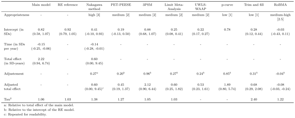
Note. The parentheses represent 95% confidence intervals.
Table P4: Publication bias correction methods (including outliers and high risk of bias studies).
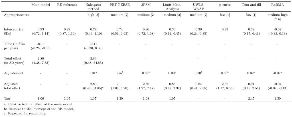
Note. The parentheses represent 95% confidence intervals.
P2.2 A note about issues in Version 3
In Version 3 we encountered a problem where our analysis that included outliers had a 70% lower (an adjustment factor of 0.30) adjusted estimate than our analysis which excluded outliers (Appendix B, Version 3). This was because the publication bias models severely corrected the effects when outliers were included. We have since increased our confidence that such severe adjustments are not appropriate (see previous sections). But, more importantly, these overcorrections were an error: In the “with-outliers” analysis of Version 3, we had incorrectly included Nakimuli-Mpungu et al. (2020, 2022) because of a coding error, a study that was meant to be excluded from every analysis (explained below).
Nakimuli-Mpungu et al. (2020, 2022) has a couple issues. It was rated as high risk of bias, in part due to the high levels of attrition and non-response. We do not include high risk of bias studies in our main analysis. But even before our risk of bias analysis we did not mean to include it (and we did not include it in neither the main nor without outliers analyses in Version 3, it was only mistakenly included in the analysis with outliers), for the following reasons. We could not extract this study’s results so its authors had to provide them to us. The data they shared implied unbelievably large effects that behaved in an unlikely manner (growing considerably over time) and the authors have not answered our follow-up questions about it. This study, if included, has an enormous amount of influence on the results (influence analysis suggested it was the main influence on the results when included) and would lead to really large results, with outliers as well as without outliers. We did not and still do not find it appropriate to include this study. Removing this study solves the problem encountered in V3.
P3. Different methods for identifying outliers
The results of an analysis can be highly influenced by outliers. Outliers can have undue influence, distort results, and inflate heterogeneity. It seemed evident to us that some effects were potential outliers. There are some extremely large effect sizes (up to ~10 SDs) with effects that are hard to believe (see Figure P1). We are unsure exactly what generated these outliers, but we are inclined to think it is related to poor study quality or statistical noise (e.g., stemming from small samples).
Figure P1: Histogram of effect sizes.
We explore multiple methods for determining outliers. There is no set way in the literature to decide what determines outliers. We tried different thresholds and methods. Overall, our choice of (g > 2 SDs) is consistent with most other methods (and conservative among them. These methods are:
- Removal based on the magnitude of the effect sizes (g > 3, g > 2.5, or g > 2)
- Removal based on median absolute deviation (MAD = 0.56) from the median effect (g = 0.59) by ±3, ±2.5, and ±2 MAD (Leys et al., 2013)
- Remove effects outside of Tukey’s fences (-1 to 2.34 gs; Tukey, 1997)
- Remove based on influence analysis where influential effect sizes are determined based on factors like Cook’s distance (Viechtbauer & Cheung, 2010), as implemented in the metafor (Viechtbauer, 2010) and the dmetar (Harrer et al.) libraries.
- Removing effect sizes whose confidence intervals do not overlap with the confidence interval of the model (Harrer et al., 2021)
Here we explore how these different methods affect our general modelling of the effect. We also explore how these affect the publication bias analysis because this is an important part of determining the effect. The results are presented in Table P5.
We are interested in the differences between the different analyses, the relative differences between these analyses and applying no outlier exclusion, and the relative differences between the analyses and the one we use in our report.
We compare the analyses on the following elements:
- How many outliers they specify and exclude.
- How big a total effect they suggest.
- The outcome of their publication bias analysis.
- The magnitude of the adjusted total effect they suggest.
- Their effect on heterogeneity.
- Their effect on model fit (AIC).
A few notes about time constraints:
- For time and computational constraints we do not include RoBMA (Bartoš et al., 2022) in our publication bias analysis for this review of the outlier analyses. This comparison could take up to 10 hours if we ran RoBMA with each of them. Furthermore, the effect of RoBMA in the more important overall alternative analyses is already discussed above. As we will demonstrate, the methods that use magnitude, MAD, or Tukey’s fences all present similar results and we do not think that RoBMA would behave differently for one or the other.
- We also do not double this analysis by conducting it with or without the high risk of bias studies. In this case we include high risk of bias studies so we can see how the methods react to all the data.
Table P5: Outliers analyses.
|
analysis |
effects excluded (included) |
τ2 |
AIC |
initial effect |
trajectory over time |
total effect |
factor relative to current analysis |
publication bias adjustment |
time adjustment |
adjusted total effect |
factor relative to current analysis |
Nakagawa method |
PET-PEESE |
3PSM |
Limit Meta-Analysis |
UWLS-WAAP |
p-curve |
Trim and fill |
|
no exclusion |
0 (361) |
1.06 |
690 |
0.93 |
-0.15 |
2.80 |
2.37 |
0.67 |
1.42 |
2.67 |
2.02 |
1.01 |
0.75 |
0.92 |
0.30 |
0.30 |
0.85 |
0.32 |
|
g > 3 |
23 (338) |
0.35 |
404 |
0.79 |
-0.17 |
1.80 |
1.53 |
0.68 |
1.48 |
1.81 |
1.37 |
0.68 |
0.73 |
0.99 |
0.60 |
0.38 |
0.97 |
0.39 |
|
g > 2.5 |
31 (330) |
0.30 |
368 |
0.77 |
-0.17 |
1.71 |
1.45 |
0.70 |
1.48 |
1.78 |
1.35 |
0.72 |
0.76 |
0.99 |
0.65 |
0.40 |
0.98 |
0.40 |
|
g > 2 |
55 (306) |
0.15 |
214 |
0.63 |
-0.18 |
1.12 |
0.95 |
0.73 |
1.53 |
1.25 |
0.95 |
0.73 |
0.75 |
0.98 |
0.71 |
0.47 |
1.06 |
0.46 |
|
MAD ± 3 |
31 (330) |
0.30 |
368 |
0.77 |
-0.17 |
1.71 |
1.45 |
0.70 |
1.48 |
1.78 |
1.35 |
0.72 |
0.76 |
0.99 |
0.65 |
0.40 |
0.98 |
0.40 |
|
MAD ± 2.5 |
45 (316) |
0.24 |
292 |
0.73 |
-0.18 |
1.45 |
1.23 |
0.71 |
1.53 |
1.57 |
1.19 |
0.71 |
0.75 |
0.98 |
0.68 |
0.43 |
1.02 |
0.43 |
|
MAD ± 2 |
57 (304) |
0.14 |
202 |
0.62 |
-0.18 |
1.07 |
0.91 |
0.73 |
1.52 |
1.19 |
0.91 |
0.72 |
0.75 |
0.97 |
0.71 |
0.47 |
1.06 |
0.46 |
|
Tukey's fences |
24 (337) |
0.34 |
396 |
0.79 |
-0.17 |
1.78 |
1.51 |
0.68 |
1.48 |
1.81 |
1.37 |
0.70 |
0.74 |
0.99 |
0.61 |
0.38 |
0.97 |
0.39 |
|
dmetar influence |
91 (270) |
1.06 |
513 |
0.83 |
-0.11 |
3.23 |
2.74 |
0.40 |
1.50 |
1.93 |
1.46 |
0.19 |
0.24 |
0.85 |
0.15 |
0.42 |
0.81 |
0.48 |
|
metafor influence |
10 (351) |
0.49 |
497 |
0.83 |
-0.17 |
2.01 |
1.70 |
0.63 |
1.47 |
1.85 |
1.41 |
0.63 |
0.68 |
0.98 |
0.48 |
0.35 |
0.93 |
0.36 |
|
non-overlapping CIs |
171 (190) |
0.07 |
147 |
0.80 |
0.05 |
20.23 |
17.14 |
4.55 |
1.00 |
91.97 |
69.80 |
16.50 |
0.92 |
1.00 |
0.94 |
0.99 |
0.90 |
1.00 |
Note. The values for the different publication bias methods are adjustment factors relative to their reference point (see Appendix E for more detail). The ‘current analysis’ is g > 2.
In Figures P2 and P3 we compare the total effects with and without time and publication bias adjustments across the different methods.
Figure P2: Total effect across the outlier analysis (before adjustments).
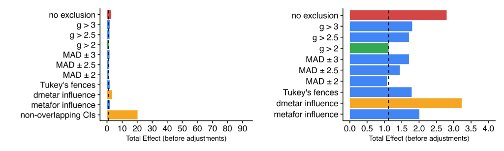
Note. The figure on the right is without the ‘non-overlapping CIs’ analysis for better readability.
Figure P3: Total effect across the outlier analysis (after time and publication bias adjustments).
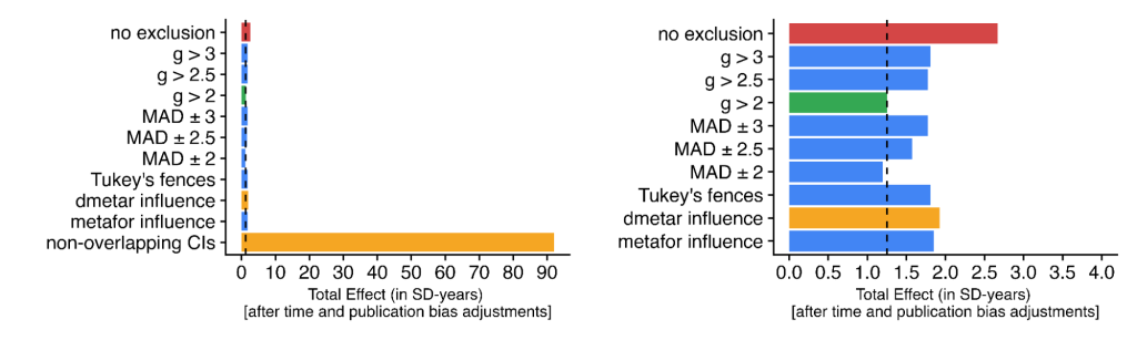
Note. The figure on the right is without the ‘non-overlapping CIs’ analysis for better readability.
We discuss three patterns which emerge from this analysis.
First, a typical method for removing outliers in meta-analysis, the non-overlapping CIs analysis (Cuijpers et al., 2020c; Harrer et al., 2021; Tong et al., 2023), performs in surprising and seemingly inappropriate ways for our analysis. It removes almost half of the effect sizes and suggests total effects that are unbelievably large. This because removing based on the confidence intervals does not account for the fact that follow-up effect might be much smaller than the average. For this reason we do not include it.
Second, we are surprised to see the dmetar and metafor influence analyses perform differently from each other. The dmetar analysis considers many more effect sizes to be influential cases, and with little overlap with metafor. Both methods calculate different Cook’s distances and attribute different weights to the effect sizes. Nevertheless, the weights of the metafor method are much closer to the weights in our modelling. The dmetar analysis considers effect sizes from studies that are seemingly high quality (Barker et al., 2022) to be influential cases but fails to detect Majidzadeh et al. (2023), which is an outlier according to all the other analyses and that we had noticed to be a likely problematic study during the extraction phase because it had extremely low error terms despite a very small sample (n = 84). It is also one of the only analyses to not substantially reduce heterogeneity. We have contacted the authors of the dmetar library for more information, meanwhile we do not consider this an appropriate outlier detection method for this report.
Third, and most importantly, the other methods (magnitude of g, MAD, Tukey’s fences, and the metafor influence analysis) perform in similar ways. Consequently, we think our choice of excluding effect sizes larger than g > 2 is not an unreasonable choice. Only the MAD ± 2 analysis reports bigger total effects than that of our chosen analysis.
We decided to exclude effect sizes larger than g > 2 for the following reasons:
- It is used in other meta-analyses authored by experts in the field (Cuijpers et al., 2020c; Tong et al., 2023).
- It is intuitive.
- Effects above this level seem hard to believe and come from studies that we informally judge to be of low quality. We think this is potentially more plausible than even the other analyses which might accept effect sizes with gs between 2 and 3.
- It gives similar results to most of the other outlier analyses.
- It is easier to explain than the other analyses.
P4. Considering only low risk of bias
In this appendix we consider whether we can run a version of our analysis with only ‘low’ risk of bias studies (k = 36, 43%). See Appendix B5 for more discussion of our risk of bias analysis.
We did not consider this our main analysis because: this loses a lot of information, not all our moderators of interest (as per Appendix G2) can be well run, a study can be considered at more risk than ‘low’ as long as one subdomain is not considered ‘low’ risk, which could be stringent, the results are not very sensitive to this, and cash transfers (our typical comparison point) do not have low risk of bias studies. The most severe way reduces the cost-effectiveness (StrongMinds: 30 WBp1k, Friendship Bench: 48 WBp1k), while the least severe way increases the cost-effectiveness (StrongMinds: 46 WBp1k, Friendship Bench: 56 WBp1k).
First, note that in our core model with both ‘low’ and ‘some concerns’ risk of bias studies, we find a moderator that suggests that ‘some concerns’ studies actually have non-significantly lower effects than (-0.05 SDs) than ‘low’ studies. When we run the model with only ‘low’ risk of bias studies it finds larger results than the main model (see Table P6). Hence, we do not expect much difference (or at least not much smaller) if we ran the whole analysis with ‘low’ risk of bias studies.
Table P6: Comparison of core modelling with different risk of bias criteria.
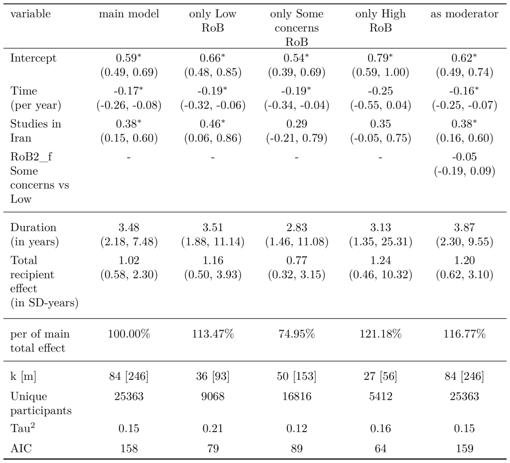
Despite the limitations above, we ran a version of our analysis with only low risk of bias studies (and excluding outliers). See Figure P4 for an illustration of the studies that are left.
Figure P4: General meta-analysis effect sizes (only low risk of bias).
Note. The colours represent different combinations of interventions and outcomes and their potential multiple effects over time (linked by a line to show their trajectory over time).
Overall, this lead to a higher total effect on the individual (2.05 → 2.36 WELLBYs). There was a harsher publication bias adjustment (0.69 → 0.53), which is surprising because we would expect that if these were better studies they would lead to less publication bias. However, there was a more positive time adjustment (i.e., the longterm follow-ups had a stronger influence; 1.54 → 1.93). On the basis of just these results and adjustments, an analysis with low risk of bias only would lead to higher results (2.18 → 2.41 WELLBYs). What was very different was the moderator adjustment because the moderators for group (-0.07 → -0.20 SDs) and lay (-0.22 → -0.43 SDs) delivery were much harsher. Overall, this reduces the cost-effectiveness of the charities (StrongMinds: 40 → 30 WBp1k, Friendship Bench: 49 → 48 WBp1k). This mainly affects StrongMinds because it is affected by the change in the group moderator.
We have reason to doubt this harsher moderating effect of group and lay delivery. If we look at the distribution of effect sizes across the moderators and risk of bias ratings (see Figure P5 and Table P7), we can see that removing ‘some concerns’ effect sizes removes a lot of information, especially about group delivery. It does not seem like ‘some concerns’ effect sizes are problematic in these distributions. For group delivery there just is very few ‘low’ risk of bias group delivery effect sizes. For lay delivery, it seems difficult to explain discounting ‘some concerns’ effect sizes when in both cases they add many lower effects, and we traditionally expect bias to increase effects in this literature. We conclude that it is more likely that the moderators estimated in our core analysis are more reliable.
Figure P5: Effect sizes for group and lay delivery according to risk of bias rating.
Table P8: Number of effect sizes for group and lay delivery according to risk of bias rating.
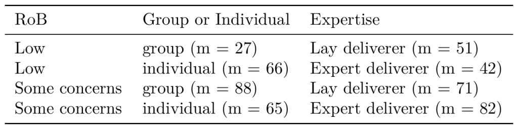
We think there are two issues with the aforementioned analysis with only ‘low’ risk of bias studies: (1) it would not be an apples-to-apples comparison to GiveDirectly (our main cost-effectiveness comparison point) because there are no ‘low’ risk of bias studies in our meta-analysis of cash transfers, and (2) it uses a moderator analysis that has too little information in it. We deal with these two points in the following manners:
- We develop that last point in detail in Appendix P4.1. One of the takeaways is that to make the comparison possible, we need to ignore some elements of the risk of bias criteria, which would increase the number of low risk of bias studies to 42 (49%) for psychotherapy (and 11, 34% for cash transfers).
- Instead of using the moderators from the ‘low’ risk of bias analysis we use those from our core analysis. So we use the change in the effect, publication bias, and time adjustment (2.05 * 0.69 * 1.54 = 2.18 → 2.31 * 0.60 * 1.89 = 2.61 WELLBYs)We calculate this as an adjustment that we add to the main analysis. but ignore the change in the moderators.
Overall, this increases the cost-effectiveness of the charities (StrongMinds: 40 → 46 WBp1k, Friendship Bench: 49 → 56 WBp1k).
We think these RoB-adjusted alternative analyses are somewhat plausible. But we think the second method we described is more appropriate. Further, we do not think it is valuable to take these at face value at the present moment. This is because these alternative analyses need to also be applied to the cash transfers analysis to make an accurate, direct comparison. This is beyond the scope of this report. Hence, even if RoB adjustments might reduce future results, the relative cost-effectiveness compared to cash transfers may be unchanged.
P4.1 Comparing risk of bias in psychotherapy and in cash transfers
Surprisingly, there was actually no ‘low’ risk of bias studies in our previously published meta-analysis of cash transfers (McGuire et al., 2022a). While our impression is that the studies in the cash transfers literature are typically higher quality, this is not reflected in the RoB ratingNote that, while this suggests that on the ‘risk of bias’ criterion the psychotherapy literature is of higher quality than the cash transfer literature, this is only one of the GRADE criteria which we use to determine quality. The cash transfers literature is higher quality than the psychotherapy literature on other criteria such as imprecision (cash transfers have larger samples and the results are more precisely estimated), inconsistency (cash transfers have lower heterogeneity), and publication bias (cash transfers have fewer publication bias issues).
.We discuss why we think that the RoB algorithm (Sterne et al., 2019) leads to lower ratings for the cash transfers literature relatively more than psychotherapy.
Any RCT that is not blinded is at a higher risk of bias. One cannot placebo getting cash (i.e., you cannot give someone something that is like money but not money without them knowing). And it is also very hard to placebo a mental health intervention but it is plausibly done with a sufficiently credible control condition. Any RCT that is not blinded is then rated as being at higher risk of bias on the 2nd domain, “deviations from the intended intervention that arose because of the trial context”. Hence, an non-blinded RCT is likely to be set at ‘some concerns’ for this domain, and thereby, its overall rating cannot be ‘low’ but, instead, has to at least be ‘some concerns’.
However, a non-blind RCT is not necessarily set as ‘some concern’ in the 2nd domain if it is reported that there were no deviations from the intended protocol. Now, cash transfers did not necessarily have a higher share of deviations from the intended intervention than for psychotherapy. There was just overwhelmingly no information provided. ‘No information’ is not treated the same as a ‘no’ in the RoB algorithm: It interprets ‘no information’ sceptically, considering that there were likely deviations and resulting in the ‘some concern’ assessment on the 2nd domain.
Why was there less reporting of information about potential deviations (or lack of)? One explanation was that there was a much greater share of natural experiments in the cash transfers literature than psychotherapy literature (~40% versus 0%), where details of implementation were not captured because the researchers were not there. Even when the cash transfers studies were RCTs, there were fewer cases of reporting.
Another explanation is that there were different raters for the cash transfers and psychotherapy literature review, and perhaps the cash transfers raters were more inclined to report ‘no information’ instead of ‘probably no’ in cases where either one was reasonable. However, while it was a long time ago, Joel (an author on this report but a rater and author in the cash transfers literature review) remembers taking a more sceptical position on cash transfers for the justifiable reason that because there were some cases where cash transfers were bundled with other interventions (e.g., a phone and bank account, access to government services) and this was not immediately clear upon first reading. Based on our understanding of psychotherapy literature, this bundling is far less common which makes a greater prevalence of ‘probably no’s instead of ‘no information’s plausibly reasonable.
This is all to say that seeking a ‘low risk of bias’ version of an analysis does not seem possible while maintaining comparable analyses for cash transfers and psychotherapy.
In our attempt to run a version of the analysis with ‘only’ low risk of bias studies we tweak the RoB algorithm to make RoB more favourable to cash transfers. We can do this by surgically setting the responses to the deviations from intended protocol to the same favourable response for both cash transfers and psychotherapy: We set the 2.3.A criteria to “No” and 2.3.B criteria to “Yes”, which leads to 42 (rather than 36) studies being considered ‘low’ risk of bias. We do not know exactly how this would affect the cash transfer study because this is outside of the scope of this report, but we think it would lead to 11 (34%) cash transfer RCTs being considered ‘low’ risk of bias.
The alternative of applying the discount only to psychotherapy – which would make it appear less favourable relative to cash transfers – seems less principled.